

Support Vector Machine using Python
In the previous article, we studied the K-Means Clustering. One thing that I believe is that if we can correlate anything with us or our lives, there are greater chances of understanding the concept. So I will try to explain everything by relating it to humans.
What is a Support Vector Machine?
Support vector machines (SVMs, also supporting vector networks) in machine learning are supervised learning models with associated learning algorithms that analyze data used for classification and regression analysis. Provided a set of training instances, each classified as belonging to one or the other of two groups, a training algorithm SVM generates a template that sells new cases for one or the other group, which renders it a non-probabilistic linear binary classifier.
A model from SVM describes the examples as points in space and is distributed to separate the examples of the different groups through a very broad void. There are then projected new instances in the same area and a range dependent on the portion of the distance in which they fall is predicted.
A hyperplane or a number of hyperplanes in a small or infinite space may be created by the support- computer and can be used for the graduation or reversal or other tasks such as the identification of outliers. The hyperplanes with the largest distance from the closest training data point of any class (so-called functional margin) intuitively achieve a good separation, as the wider the margin, the lower the generalization error of the classification system.
Note:
When data are unlisted, supervised education is not available and there is a need for an unsupervised learning approach that attempts to find a natural grouping of data and then map new data to the groups that are formed.
Key Terms
-
Kernel
- A kernel refers to a feature that converts the data into a wide space for solving the problem.
- A linear or non-linear kernel function may be used. Kernel methods are a type of pattern analysis algorithm.
- The kernel's primary role is to accept data as input and convert it into the appropriate output types.
- In statistics, the mapping feature "core" measures the values of two-dominal data in a three-dimensional spatial format and describes them.
-
Regularization
- The regularization function is also named the C function in the sklearn library of python, which guides the help vector machine to optimally define each training date it wants to prevent.
- Such a supporting vector machine example will auto-optimization if large numbers of the C parameter are used if all training data points are correctly segregated and classification is collected the hyperplanes margin that is smaller.
- To order to obtain very tiny numbers, the algorithm can often consider that the hyperplane is a larger range and certain data points may be misclassified by the hyperplane.
-
Gamma
- This tuning function reiterates the length of the effect of a single data display. The low values are 'far' and the higher values are 'near' to the aircraft.
- In measurement for a separation line, the data points with low gamma are called and are far from the possible hyper-plane separation line.
- In comparison, the high range is used in the measurement of the hyper-plane separation line which applies to the points that are similar to the expected hyper-plane line.
-
Margin
- The gap is last but not least. It's also a significant tuning parameter & an integral function of a vector holder classification system.
- The margin is the division of the line closest to the data points of the segment. In a support vector algorithm, it is necessary to have a good and proper margin. When the difference between the two data groups is greater, a strong gap is called.
- To a strong range, the corresponding data points stay in class and thus do not move over to another level.
- Also, the class data points will have a reasonable margin preferably at the same distance from either side of the separator panel.
-
Hyperplane
- A hyperplane is a linear, n-1 dimensional subset of this space, which splits the space into two divided parts in an n-dimensional Euclidean space.
- For two dimensions the hyperplane is a separating line.
- For three dimensions a plane with two dimensions divides the 3d space into two parts and thus acts as a hyperplane.
- Thus for a space of n dimensions, we have a hyperplane of n-1 dimensions separating it into two parts.
Types of SVM
- Classification SVM type 1 (also known as C-SVM classification)
- Classification SVM type 2 (also known as nu-SVM classification)
- Regression SVM type 1 (also known as epsilon-SVM regression)
- Regression SVM type 2 (also known as nu-SVM regression)
Types of kernels
- Linear kernel
- Polynomial kernel
- Radial basis function kernel (RBF)/ Gaussian Kernel
- Sigmoid Kernel
- Nonlinear Kernel
Advantages/Features of SVM
- It is really effective in a higher dimension.
- Effective when the number of features is more than training examples.
- Best algorithm when classes are separable
- The hyperplane is affected by only the support vectors thus outliers have less impact.
- SVM is suited for extreme case binary classification.
Disadvantages/Shortcomings of SVM
- For the larger dataset, it requires a large amount of time to process.
- It does not perform well in case of overlapped classes.
- Selecting, appropriately hyperparameters of the SVM that will allow for sufficient generalization performance.
- Selecting the appropriate kernel function can be tricky.
Real-World Applications of SVM
- Face detection
SVM classifies parts of the image as a face and non-face and creates a square boundary around the face.
- Text and hypertext categorization
SVMs allow Text and hypertext categorization for both inductive and transductive models. They use training data to classify documents into different categories. It categorizes on the basis of the score generated and then compares with the threshold value.
- Classification of images
Use of SVMs provides better search accuracy for image classification. It provides better accuracy in comparison to the traditional query-based searching techniques.
- Bioinformatics
It includes protein classification and cancer classification. We use SVM for identifying the classification of genes, patients on the basis of genes and other biological problems.
- Protein fold and remote homology detection
Apply SVM algorithms for protein remote homology detection.
- Handwriting recognition
We use SVMs to recognize handwritten characters used widely.
- Generalized predictive control(GPC)
Use SVM based GPC to control chaotic dynamics with useful parameters.
SVM using Example
Like in other ML algorithms we find the best fit, in SVM we try to find a hyperplane with the maximum margin or distance, hence it is also a type of "maximum-margin" classification.
Let us try to understand SVM with the help of a mathematical example, for this example,
| Data Points | Class |
| (-2, 4) | -1 |
| (4,1) | -1 |
| (1,6) | 1 |
| (2,4) | 1 |
| (6,2) | 1 |
Now before I go on further I want you to first know:
1. Hinge loss
In machine learning, the hinge loss is a loss function used for training classifiers. The hinge loss is used for "maximum-margin" classification, most notably for support vector machines (SVMs).
The equation is given as:
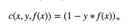
where c is the loss function, x the sample, y is the true label, f(x) the predicted label.
You see a plus at the end, it means that the hinge error can never be negative, mathematically I can be expressed as:

2. Regularizer
The regularizer balances between margin maximization and loss. The regularizer controls the trade-off between achieving a low training error and a low testing error that is the ability to generalize your classifier to unseen data. As a regularizing parameter we choose 1/epochs, so this parameter will decrease, as the number of epochs increases.
Regularixer, λ = 1/epoch
3. Weight Vector
The SVM algorithm chooses a particular weight vector, that which gives rise to the “maximum margin” of separation
Now coming back to the math of SVM, generation of the hyperplane we can have 2 scenarios
1. Misclassification, i.e. the point is not classified correctly
2. Correct Classification
In the case of misclassification, we use the following to update the weights:

and in case of correct classification, we use the following to update the weights:

where,
- η is the learning rate
- λ is the regularizer
After doing the calculations, I came up with the following prediction function:
f(x) = (x, (1.56, 3.17))- 11.12
i.e f(x) = 1.56*x + 3.17*y -11.12
where,
- (1.56, 3.17) is the weight vector
- 11.12 is the bias term
Note: I will not be going into depth on how I got this, you can do the calculations by yourself or you can use sklearn to do it for you.
Now let us check the accuracy of the prediction function so calculated
1. -2*1.56 + 4*3.17 - 11.12
= -1.56
taking the sign out, we get -1, which is the correct class
2. 4*1.56 + 1*3.17 - 11.12
= -1.72
taking the sign out, we get -1, which is the correct class
3. 1*1.56 + 6*3.17 - 11.12
= 9.46
taking the sign out, we get +1, which is the correct class
4. 2*1.56 + 4*3.17 - 11.12
= 4.68
taking the sign out, we get +1, which is the correct class
5. 6*1.56 + 2*3.17 - 11.12
= 4.58
taking the sign out, we get +1, which is the correct class
So until now, we tested the hyperplane equation on the training data. Now its time to give some never seen before data to the model
Test Data = (3, 5), (-2, 3)
1. 3*1.56 + 5*3.17 - 11.12
= 9.41
Taking the sign out, we get +1, which is the correct class
2. -2*1.56 + 3*3.17 - 11.12
= -4.73
Taking the sign out, we get -1, which is the correct class
Python Implementation of SVM
1. Using Functions
Let us now take a look at how can we implement SVM from scratch. In the following example, we will take dummy data. I have taken the code reference from the repository.
- # importing some basic libraries
- %matplotlib inline
- import matplotlib.pyplot as plt
- from matplotlib import style
- style.use('ggplot')
- import numpy as np
- class SVM(object):
- def __init__(self,visualization=True):
- self.visualization = visualization
- self.colors = {1:'r',-1:'b'}
- if self.visualization:
- self.fig = plt.figure()
- self.ax = self.fig.add_subplot(1,1,1)
- def fit(self,data):
- #train with data
- self.data = data
- # { |\w\|:{w,b}}
- opt_dict = {}
- transforms = [[1,1],[-1,1],[-1,-1],[1,-1]]
- all_data = np.array([])
- for yi in self.data:
- all_data = np.append(all_data,self.data[yi])
- self.max_feature_value = max(all_data)
- self.min_feature_value = min(all_data)
- all_data = None
- #with smaller steps our margins and db will be more precise
- step_sizes = [self.max_feature_value * 0.1,
- self.max_feature_value * 0.01,
- #point of expense
- self.max_feature_value * 0.001,]
- #extremly expensise
- b_range_multiple = 5
- #we dont need to take as small step as w
- b_multiple = 5
- latest_optimum = self.max_feature_value*10
- """
- objective is to satisfy yi(x.w)+b>=1 for all training dataset such that ||w|| is minimum
- for this we will start with random w, and try to satisfy it with making b bigger and bigger
- """
- #making step smaller and smaller to get precise value
- for step in step_sizes:
- w = np.array([latest_optimum,latest_optimum])
- #we can do this because convex
- optimized = False
- while not optimized:
- for b in np.arange(-1*self.max_feature_value*b_range_multiple,
- self.max_feature_value*b_range_multiple,
- step*b_multiple):
- for transformation in transforms:
- w_t = w*transformation
- found_option = True
- #weakest link in SVM fundamentally
- #SMO attempts to fix this a bit
- # ti(xi.w+b) >=1
- for i in self.data:
- for xi in self.data[i]:
- yi=i
- if not yi*(np.dot(w_t,xi)+b)>=1:
- found_option=False
- if found_option:
- """
- all points in dataset satisfy y(w.x)+b>=1 for this cuurent w_t, b
- then put w,b in dict with ||w|| as key
- """
- opt_dict[np.linalg.norm(w_t)]=[w_t,b]
- #after w[0] or w[1]<0 then values of w starts repeating itself because of transformation
- #Think about it, it is easy
- #print(w,len(opt_dict)) Try printing to understand
- if w[0]<0:
- optimized=True
- print("optimized a step")
- else:
- w = w-step
- # sorting ||w|| to put the smallest ||w|| at poition 0
- norms = sorted([n for n in opt_dict])
- #optimal values of w,b
- opt_choice = opt_dict[norms[0]]
- self.w=opt_choice[0]
- self.b=opt_choice[1]
- #start with new latest_optimum (initial values for w)
- latest_optimum = opt_choice[0][0]+step*2
- def predict(self,features):
- #sign(x.w+b)
- classification = np.sign(np.dot(np.array(features),self.w)+self.b)
- if classification!=0 and self.visualization:
- self.ax.scatter(features[0],features[1],s=200,marker='*',c=self.colors[classification])
- return (classification,np.dot(np.array(features),self.w)+self.b)
- def visualize(self):
- [[self.ax.scatter(x[0],x[1],s=100,c=self.colors[i]) for x in data_dict[i]] for i in data_dict]
- # hyperplane = x.w+b (actually its a line)
- # v = x0.w0+x1.w1+b -> x1 = (v-w[0].x[0]-b)/w1
- #psv = 1 psv line -> x.w+b = 1a small value of b we will increase it later
- #nsv = -1 nsv line -> x.w+b = -1
- # dec = 0 db line -> x.w+b = 0
- def hyperplane(x,w,b,v):
- #returns a x2 value on line when given x1
- return (-w[0]*x-b+v)/w[1]
- hyp_x_min= self.min_feature_value*0.9
- hyp_x_max = self.max_feature_value*1.1
- # (w.x+b)=1
- # positive support vector hyperplane
- pav1 = hyperplane(hyp_x_min,self.w,self.b,1)
- pav2 = hyperplane(hyp_x_max,self.w,self.b,1)
- self.ax.plot([hyp_x_min,hyp_x_max],[pav1,pav2],'k')
- # (w.x+b)=-1
- # negative support vector hyperplane
- nav1 = hyperplane(hyp_x_min,self.w,self.b,-1)
- nav2 = hyperplane(hyp_x_max,self.w,self.b,-1)
- self.ax.plot([hyp_x_min,hyp_x_max],[nav1,nav2],'k')
- # (w.x+b)=0
- # db support vector hyperplane
- db1 = hyperplane(hyp_x_min,self.w,self.b,0)
- db2 = hyperplane(hyp_x_max,self.w,self.b,0)
- self.ax.plot([hyp_x_min,hyp_x_max],[db1,db2],'y--')
- #defining a basic data
- data_dict = {-1:np.array([[1,7],[2,8],[3,8]]),1:np.array([[5,1],[6,-1],[7,3]])}
- svm = SVM() # Linear Kernel
- svm.fit(data=data_dict)
- svm.visualize()
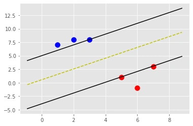
- svm.predict([3,8])
OUTPUT
(-1.0, -1.000000000000098)
2. Using Sklearn
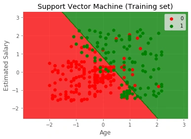
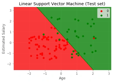
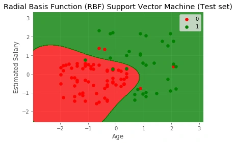
Let us now take a look at how can we implement SVM using sklearn. In the following example, I have used Social Network data, please find it attached. I have taken the code reference from the repository.
- # Importing the libraries
- import numpy as np
- import matplotlib.pyplot as plt
- import pandas as pd
- # Importing the datasets
- datasets = pd.read_csv('Social_Network_Ads.csv')
- X = datasets.iloc[:, [2,3]].values
- Y = datasets.iloc[:, 4].values
- # Splitting the dataset into the Training set and Test set
- from sklearn.model_selection import train_test_split
- X_Train, X_Test, Y_Train, Y_Test = train_test_split(X, Y, test_size = 0.25, random_state = 0)
- # Feature Scaling
- from sklearn.preprocessing import StandardScaler
- sc_X = StandardScaler()
- X_Train = sc_X.fit_transform(X_Train)
- X_Test = sc_X.transform(X_Test)
- # Fitting the classifier into the Training set
- from sklearn.svm import SVC
- classifier = SVC(kernel = 'linear', random_state = 0)
- classifier.fit(X_Train, Y_Train)
- # Predicting the test set results
- Y_Pred = classifier.predict(X_Test)
- # Making the Confusion Matrix
- from sklearn.metrics import confusion_matrix
- cm = confusion_matrix(Y_Test, Y_Pred)
- # Visualising the Training set results
- from matplotlib.colors import ListedColormap
- X_Set, Y_Set = X_Train, Y_Train
- X1, X2 = np.meshgrid(np.arange(start = X_Set[:, 0].min() - 1, stop = X_Set[:, 0].max() + 1, step = 0.01),
- np.arange(start = X_Set[:, 1].min() - 1, stop = X_Set[:, 1].max() + 1, step = 0.01))
- plt.contourf(X1, X2, classifier.predict(np.array([X1.ravel(), X2.ravel()]).T).reshape(X1.shape),
- alpha = 0.75, cmap = ListedColormap(('red', 'green')))
- plt.xlim(X1.min(), X1.max())
- plt.ylim(X2.min(), X2.max())
- for i, j in enumerate(np.unique(Y_Set)):
- plt.scatter(X_Set[Y_Set == j, 0], X_Set[Y_Set == j, 1],
- c = ListedColormap(('red', 'green'))(i), label = j)
- plt.title('Support Vector Machine (Training set)')
- plt.xlabel('Age')
- plt.ylabel('Estimated Salary')
- plt.legend()
- plt.show()
- # Visualising the Test set results
- from matplotlib.colors import ListedColormap
- X_Set, Y_Set = X_Test, Y_Test
- X1, X2 = np.meshgrid(np.arange(start = X_Set[:, 0].min() - 1, stop = X_Set[:, 0].max() + 1, step = 0.01),
- np.arange(start = X_Set[:, 1].min() - 1, stop = X_Set[:, 1].max() + 1, step = 0.01))
- plt.contourf(X1, X2, classifier.predict(np.array([X1.ravel(), X2.ravel()]).T).reshape(X1.shape),
- alpha = 0.75, cmap = ListedColormap(('red', 'green')))
- plt.xlim(X1.min(), X1.max())
- plt.ylim(X2.min(), X2.max())
- for i, j in enumerate(np.unique(Y_Set)):
- plt.scatter(X_Set[Y_Set == j, 0], X_Set[Y_Set == j, 1],
- c = ListedColormap(('red', 'green'))(i), label = j)
- plt.title('Linear Support Vector Machine (Test set)')
- plt.xlabel('Age')
- plt.ylabel('Estimated Salary')
- plt.legend()
- plt.show()
- from sklearn.svm import SVC
- classifier = SVC(kernel = 'rbf', random_state = 0)
- classifier.fit(X_Train, Y_Train)
- # Predicting the test set results
- Y_Pred = classifier.predict(X_Test)
- # Making the Confusion Matrix
- from sklearn.metrics import confusion_matrix
- cm = confusion_matrix(Y_Test, Y_Pred)
- # Visualising the Test set results
- from matplotlib.colors import ListedColormap
- X_Set, Y_Set = X_Test, Y_Test
- X1, X2 = np.meshgrid(np.arange(start = X_Set[:, 0].min() - 1, stop = X_Set[:, 0].max() + 1, step = 0.01),
- np.arange(start = X_Set[:, 1].min() - 1, stop = X_Set[:, 1].max() + 1, step = 0.01))
- plt.contourf(X1, X2, classifier.predict(np.array([X1.ravel(), X2.ravel()]).T).reshape(X1.shape),
- alpha = 0.75, cmap = ListedColormap(('red', 'green')))
- plt.xlim(X1.min(), X1.max())
- plt.ylim(X2.min(), X2.max())
- for i, j in enumerate(np.unique(Y_Set)):
- plt.scatter(X_Set[Y_Set == j, 0], X_Set[Y_Set == j, 1],
- c = ListedColormap(('red', 'green'))(i), label = j)
- plt.title('Radial Basis Function (RBF) Support Vector Machine (Test set)')
- plt.xlabel('Age')
- plt.ylabel('Estimated Salary')
- plt.legend()
- plt.show()
OUTPUT
3. Using Tensorflow
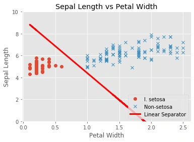
Let us now take a look at how can we implement SVM using TensorFlow. In the following example, I am using the IRIS dataset. I have taken the code reference from the repository.
Note: tf.disable_v2_behaviour() is used to use the Tensorflow 1 functionalities, as i have Tensorflow 2 installed on my PC.
- import matplotlib.pyplot as plt
- import numpy as np
- import tensorflow.compat.v1 as tf
- tf.disable_v2_behavior()
- from sklearn import datasets
- from tensorflow.python.framework import ops
- ops.reset_default_graph()
- # Set random seeds
- np.random.seed(7)
- tf.set_random_seed(7)
- # Create graph
- sess = tf.Session()
- # Load the data
- # iris.data = [(Sepal Length, Sepal Width, Petal Length, Petal Width)]
- iris = datasets.load_iris()
- x_vals = np.array([[x[0], x[3]] for x in iris.data])
- y_vals = np.array([1 if y == 0 else -1 for y in iris.target])
- # Split data into train/test sets
- train_indices = np.random.choice(len(x_vals),
- int(round(len(x_vals)*0.9)),
- replace=False)
- test_indices = np.array(list(set(range(len(x_vals))) - set(train_indices)))
- x_vals_train = x_vals[train_indices]
- x_vals_test = x_vals[test_indices]
- y_vals_train = y_vals[train_indices]
- y_vals_test = y_vals[test_indices]
- # Declare batch size
- batch_size = 135
- # Initialize placeholders
- x_data = tf.placeholder(shape=[None, 2], dtype=tf.float32)
- y_target = tf.placeholder(shape=[None, 1], dtype=tf.float32)
- # Create variables for linear regression
- A = tf.Variable(tf.random_normal(shape=[2, 1]))
- b = tf.Variable(tf.random_normal(shape=[1, 1]))
- # Declare model operations
- model_output = tf.subtract(tf.matmul(x_data, A), b)
- # Declare vector L2 'norm' function squared
- l2_norm = tf.reduce_sum(tf.square(A))
- # Declare loss function
- # Loss = max(0, 1-pred*actual) + alpha * L2_norm(A)^2
- # L2 regularization parameter, alpha
- alpha = tf.constant([0.01])
- # Margin term in loss
- classification_term = tf.reduce_mean(tf.maximum(0., tf.subtract(1., tf.multiply(model_output, y_target))))
- # Put terms together
- loss = tf.add(classification_term, tf.multiply(alpha, l2_norm))
- # Declare prediction function
- prediction = tf.sign(model_output)
- accuracy = tf.reduce_mean(tf.cast(tf.equal(prediction, y_target), tf.float32))
- # Declare optimizer
- my_opt = tf.train.GradientDescentOptimizer(0.01)
- train_step = my_opt.minimize(loss)
- # Initialize variables
- init = tf.global_variables_initializer()
- sess.run(init)
- # Training loop
- loss_vec = []
- train_accuracy = []
- test_accuracy = []
- for i in range(500):
- rand_index = np.random.choice(len(x_vals_train), size=batch_size)
- rand_x = x_vals_train[rand_index]
- rand_y = np.transpose([y_vals_train[rand_index]])
- sess.run(train_step, feed_dict={x_data: rand_x, y_target: rand_y})
- temp_loss = sess.run(loss, feed_dict={x_data: rand_x, y_target: rand_y})
- loss_vec.append(temp_loss)
- train_acc_temp = sess.run(accuracy, feed_dict={
- x_data: x_vals_train,
- y_target: np.transpose([y_vals_train])})
- train_accuracy.append(train_acc_temp)
- test_acc_temp = sess.run(accuracy, feed_dict={
- x_data: x_vals_test,
- y_target: np.transpose([y_vals_test])})
- test_accuracy.append(test_acc_temp)
- if (i + 1) % 100 == 0:
- print('Step #{} A = {}, b = {}'.format(
- str(i+1),
- str(sess.run(A)),
- str(sess.run(b))
- ))
- print('Loss = ' + str(temp_loss))
- # Extract coefficients
- [[a1], [a2]] = sess.run(A)
- [[b]] = sess.run(b)
- slope = -a2/a1
- y_intercept = b/a1
- # Extract x1 and x2 vals
- x1_vals = [d[1] for d in x_vals]
- # Get best fit line
- best_fit = []
- for i in x1_vals:
- best_fit.append(slope*i+y_intercept)
- # Separate I. setosa
- setosa_x = [d[1] for i, d in enumerate(x_vals) if y_vals[i] == 1]
- setosa_y = [d[0] for i, d in enumerate(x_vals) if y_vals[i] == 1]
- not_setosa_x = [d[1] for i, d in enumerate(x_vals) if y_vals[i] == -1]
- not_setosa_y = [d[0] for i, d in enumerate(x_vals) if y_vals[i] == -1]
- # Plot data and line
- plt.plot(setosa_x, setosa_y, 'o', label='I. setosa')
- plt.plot(not_setosa_x, not_setosa_y, 'x', label='Non-setosa')
- plt.plot(x1_vals, best_fit, 'r-', label='Linear Separator', linewidth=3)
- plt.ylim([0, 10])
- plt.legend(loc='lower right')
- plt.title('Sepal Length vs Petal Width')
- plt.xlabel('Petal Width')
- plt.ylabel('Sepal Length')
- plt.show()
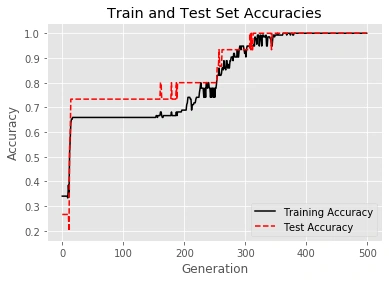
- # Plot train/test accuracies
- plt.plot(train_accuracy, 'k-', label='Training Accuracy')
- plt.plot(test_accuracy, 'r--', label='Test Accuracy')
- plt.title('Train and Test Set Accuracies')
- plt.xlabel('Generation')
- plt.ylabel('Accuracy')
- plt.legend(loc='lower right')
- plt.show()
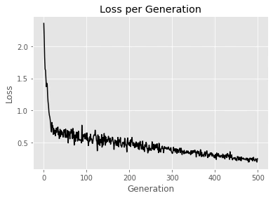
- # Plot loss over time
- plt.plot(loss_vec, 'k-')
- plt.title('Loss per Generation')
- plt.xlabel('Generation')
- plt.ylabel('Loss')
- plt.show()
OUTPUT
Step #100 A = [[-0.4810509 ]
[ 0.05859518]], b = [[-1.8697345]]
Loss = [0.64420575]
Step #200 A = [[-0.4076391 ]
[-0.25413615]], b = [[-1.9181045]]
Loss = [0.45963168]
Step #300 A = [[-0.34309638]
[-0.55148035]], b = [[-1.9694378]]
Loss = [0.34777495]
Step #400 A = [[-0.28505743]
[-0.83066034]], b = [[-2.023808]]
Loss = [0.25850892]
Step #500 A = [[-0.22314341]
[-1.096483 ]], b = [[-2.0792139]]
Loss = [0.2473848]
Conclusion
In this article, we studied support vector machine, key terms of SVM, types of SVM, types of SVM kernels, advantages and disadvantages of SVM, real-world applications of SVM, SVM explanation using an example, and python implementation of the SVM algorithm using functions, sklearn, and TensorFlow. Hope you were able to understand everything. For any doubts, please comment on your query.
Congratulations!!! You have climbed your next step in becoming a successful ML Engineer.
Ashish BhatnagarPosted Dec 31, 2021, 10:51 AM
Very Informative and Perfect Article on SVM....
Rijwan AnsariPosted Feb 3, 2021, 1:36 PM
Informative and rich article...
Chaman GautamPosted Apr 22, 2020, 4:12 AM
Nice article sir