SQL Server Features: A Comprehensive Guide for Developers

SQL

Image source: online

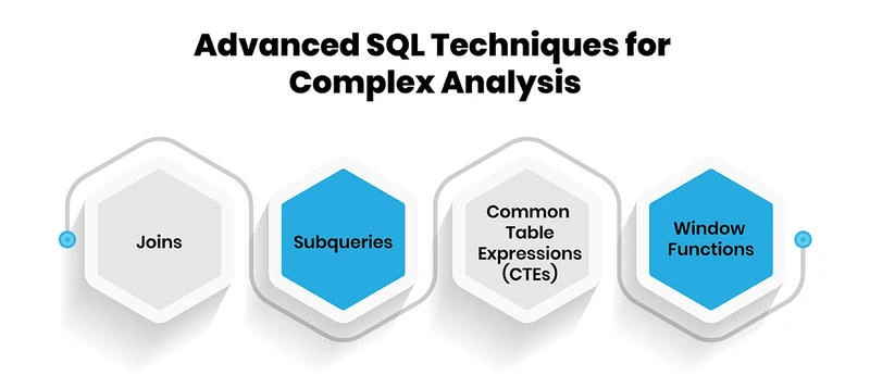
In this article, we’ll dive deep into ten powerful SQL Server features: Common Table Expressions (CTEs), Window Functions, LATERAL Joins (CROSS APPLY / OUTER APPLY), GROUPING SETS, ROLLUP & CUBE, FILTER Clause in Aggregates, UPSERT (MERGE / INSERT...ON CONFLICT), JSON Support & JSON_TABLE, Computed / Generated Columns, TABLESAMPLE, and Partial Indexes.

For each feature, we’ll explore:

What it is: A clear definition and purpose.
Basic to Advanced Examples: Starting with simple use cases and progressing to complex scenarios.
Example Data: Sample datasets to illustrate functionality.
Scenarios: Real-world applications of the feature.
Alternatives: Other ways to achieve similar results.
Usage Cases: Practical contexts where the feature shines.
Performance Issues: Potential bottlenecks and optimization tips.
Pros and Cons: Benefits and limitations.
Business Case: How the feature solves business problems.

This article assumes familiarity with SQL Server, given your experience since 2009, but it’s structured to be accessible while diving into advanced applications. Let’s get started!

Table of Contents

Common Table Expressions (CTEs) (#common-table-expressions-ctes)
Window Functions (#window-functions)
LATERAL Joins (CROSS APPLY / OUTER APPLY) (#lateral-joins-cross-apply--outer-apply)
GROUPING SETS, ROLLUP & CUBE (#grouping-sets-rollup--cube)
FILTER Clause in Aggregates (#filter-clause-in-aggregates)
UPSERT (MERGE / INSERT...ON CONFLICT) (#upsert-merge--inserton-conflict)
JSON Support & JSON_TABLE (#json-support--json_table)
Computed / Generated Columns (#computed--generated-columns)
TABLESAMPLE (#tablesample)
Partial Indexes (#partial-indexes)
Conclusion (#conclusion)

Common Table Expressions (CTEs)

What are CTEs?

Common Table Expressions (CTEs) are temporary result sets defined within a SQL query’s scope, allowing you to name and reuse a subquery multiple times in a single query. Introduced in SQL Server 2005, CTEs improve query readability and maintainability, especially for complex operations like recursive queries.Basic ExampleLet’s start with a simple CTE to calculate total sales per employee.

-- Sample Data
CREATE TABLE Sales (
    EmployeeID INT,
    SaleAmount DECIMAL(10, 2),
    SaleDate DATE
);
INSERT INTO Sales (EmployeeID, SaleAmount, SaleDate)
VALUES (1, 500.00, '2025-01-01'), (1, 300.00, '2025-01-02'),
       (2, 700.00, '2025-01-01'), (2, 200.00, '2025-01-03');

-- Basic CTE
WITH EmployeeSales AS (
    SELECT EmployeeID, SUM(SaleAmount) AS TotalSales
    FROM Sales
    GROUP BY EmployeeID
)
SELECT EmployeeID, TotalSales
FROM EmployeeSales
WHERE TotalSales > 500;

Output

EmployeeID | TotalSales
-----------|-----------
1          | 800.00
2          | 900.00

Advanced Example: Recursive CTERecursive CTEs are powerful for hierarchical data, such as organizational charts.

-- Sample Data: Employee Hierarchy
CREATE TABLE Employees (
    EmployeeID INT PRIMARY KEY,
    EmployeeName VARCHAR(50),
    ManagerID INT
);
INSERT INTO Employees (EmployeeID, EmployeeName, ManagerID)
VALUES (1, 'CEO', NULL), (2, 'Manager A', 1), (3, 'Manager B', 1),
       (4, 'Employee A1', 2), (5, 'Employee A2', 2), (6, 'Employee B1', 3);

-- Recursive CTE to build hierarchy
WITH EmployeeHierarchy AS (
    -- Anchor Member: Start with the CEO
    SELECT EmployeeID, EmployeeName, ManagerID, 0 AS Level
    FROM Employees
    WHERE ManagerID IS NULL
    UNION ALL
    -- Recursive Member: Get subordinates
    SELECT e.EmployeeID, e.EmployeeName, e.ManagerID, eh.Level + 1
    FROM Employees e
    INNER JOIN EmployeeHierarchy eh ON e.ManagerID = eh.EmployeeID
)
SELECT EmployeeID, EmployeeName, ManagerID, Level
FROM EmployeeHierarchy
ORDER BY Level, EmployeeName;

Output

EmployeeID | EmployeeName | ManagerID | Level
-----------|-------------|-----------|------
1          | CEO         | NULL      | 0
2          | Manager A   | 1         | 1
3          | Manager B   | 1         | 1
4          | Employee A1 | 2         | 2
5          | Employee A2 | 2         | 2
6          | Employee B1 | 3         | 2

Scenarios

Reporting: Summarize data hierarchically, e.g., sales by region and subregion.
Data Cleaning: Break down complex transformations into readable steps.
Recursive Queries: Navigate tree-like structures, such as bill-of-materials or organizational charts.

Alternatives

Subqueries: Inline subqueries can replace simple CTEs but are less readable.
Temporary Tables: Store intermediate results but require more setup and cleanup.
Views: Permanent storage for reusable queries but less flexible for ad-hoc analysis.

Usage Cases

Hierarchical Data: Organizational charts, product categories, or file systems.
Complex Aggregations: Break down multi-step calculations in reports.
Query Refactoring: Simplify nested subqueries for better maintainability.

Performance Issues

Recursive CTEs: Can be slow for deep hierarchies due to iterative processing. Ensure proper indexing on joining columns (e.g., ManagerID).
Large Datasets: CTEs materialize results in memory; for massive datasets, temporary tables might perform better.
Optimization: Use indexes on columns used in CTE filters or joins to improve performance.

Pros and ConsPros

Enhances query readability and maintainability.
Supports recursion for hierarchical data.
Reusable within the same query scope.

Cons

Not reusable across multiple queries (unlike views).
Recursive CTEs can be resource-intensive for deep hierarchies.
Materialization may impact performance with large datasets.

Business Case Scenario: A retail company needs to analyze its organizational structure to assess reporting lines for a compensation review. A recursive CTE can map the hierarchy from CEO to entry-level employees, enabling HR to calculate bonuses based on levels or reporting chains. This approach is faster and more maintainable than manual reporting or multiple subqueries, saving time and reducing errors.

Window Functions

What are Window Functions?

Window Functions perform calculations across a set of rows (a “window”) related to the current row, without collapsing the result set like aggregates do. Introduced in SQL Server 2005 and enhanced in 2012, they’re ideal for ranking, running totals, and moving averages.Basic ExampleCalculate a running total of sales per employee.

-- Using Sales table from CTE example
SELECT EmployeeID, SaleAmount, SaleDate,
       SUM(SaleAmount) OVER (PARTITION BY EmployeeID ORDER BY SaleDate) AS RunningTotal
FROM Sales;

Output

EmployeeID | SaleAmount | SaleDate   | RunningTotal
-----------|------------|------------|-------------
1          | 500.00     | 2025-01-01 | 500.00
1          | 300.00     | 2025-01-02 | 800.00
2          | 700.00     | 2025-01-01 | 700.00
2          | 200.00     | 2025-01-03 | 900.00

Advanced Example: Ranking with Tie HandlingRank employees by sales within each month, handling ties with DENSE_RANK.

SELECT EmployeeID, SaleAmount, SaleDate,
       DENSE_RANK() OVER (PARTITION BY MONTH(SaleDate) ORDER BY SaleAmount DESC) AS SalesRank
FROM Sales
WHERE YEAR(SaleDate) = 2025;

Output (assuming more data)

EmployeeID | SaleAmount | SaleDate   | SalesRank
-----------|------------|------------|----------
2          | 700.00     | 2025-01-01 | 1
1          | 500.00     | 2025-01-01 | 2
1          | 300.00     | 2025-01-02 | 3
2          | 200.00     | 2025-01-03 | 4

Scenarios

Financial Reporting: Calculate running totals or moving averages for budgeting.
Leaderboard Systems: Rank users by performance metrics (e.g., sales, scores).
Data Analysis: Compute percentiles or compare rows within groups.

Alternatives

Self-Joins: Achieve similar results but are less efficient and harder to read.
Subqueries: Can calculate row-specific aggregates but are verbose.
Cursors: Process rows iteratively but are slow and resource-heavy.

Usage Cases

Running Totals: Track cumulative sales or inventory over time.
Ranking: Identify top performers in sales or customer engagement.
Lag/Lead Analysis: Compare current row values with previous or next rows (e.g., stock price changes).

Performance Issues

Window Size: Large partitions (e.g., millions of rows) can slow queries. Use filtered indexes or partition tables.
Sorting: ORDER BY in OVER clause can be costly; ensure indexes on sorted columns.
Memory Usage: Window functions may spill to disk for large datasets, impacting performance.

Pros and Cons

Pros

Perform complex calculations without collapsing rows.
Highly flexible for analytics (ranking, aggregates, etc.).
Clean syntax compared to alternatives.

Cons

Can be resource-intensive for large datasets.
Requires understanding of window definitions.
Limited to row-based calculations within a query.

Business Case Scenario: A sales team wants to identify top performers monthly to allocate bonuses. Using DENSE_RANK with window functions, the company can rank employees by sales within each month, automatically handling ties and providing clear insights for incentive programs. This avoids complex self-joins and improves query performance.

LATERAL Joins (CROSS APPLY / OUTER APPLY)

What are LATERAL Joins?

CROSS APPLY and OUTER APPLY, introduced in SQL Server 2005, allow a subquery or table-valued function to reference columns from the outer query, acting like a correlated subquery but with set-based processing. They’re SQL Server’s equivalent of LATERAL joins in other databases.

Basic Example: Retrieve the top 2 sales per employee.

SELECT e.EmployeeID, s.SaleAmount, s.SaleDate
FROM Employees e
CROSS APPLY (
    SELECT TOP 2 SaleAmount, SaleDate
    FROM Sales s
    WHERE s.EmployeeID = e.EmployeeID
    ORDER BY SaleAmount DESC
) s;

Output

EmployeeID | SaleAmount | SaleDate
-----------|------------|------------
1          | 500.00     | 2025-01-01
1          | 300.00     | 2025-01-02
2          | 700.00     | 2025-01-01
2          | 200.00     | 2025-01-03

Advanced Example: Table-Valued FunctionUse a table-valued function to calculate sales metrics.

CREATE FUNCTION dbo.GetSalesMetrics (@EmployeeID INT)
RETURNS TABLE AS
RETURN (
    SELECT SUM(SaleAmount) AS TotalSales, COUNT(*) AS SaleCount
    FROM Sales
    WHERE EmployeeID = @EmployeeID
);

SELECT e.EmployeeID, e.EmployeeName, sm.TotalSales, sm.SaleCount
FROM Employees e
CROSS APPLY dbo.GetSalesMetrics(e.EmployeeID) sm;

Output

EmployeeID | EmployeeName | TotalSales | SaleCount
-----------|-------------|------------|----------
1          | CEO         | NULL       | 0
2          | Manager A   | 800.00     | 2
3          | Manager B   | 900.00     | 2

Scenarios

Dynamic Subqueries: Fetch related data per row, e.g., top-N records.
Function Integration: Apply table-valued functions to each row.
Complex Joins: Combine data where traditional joins are insufficient.

Alternatives

Correlated Subqueries: Similar but often slower and less readable.
Derived Tables: Can mimic APPLY but are less flexible.
CTEs: Can structure subqueries but lack row-by-row correlation.

Usage Cases

Top-N Queries: Retrieve top sales, orders, or events per group.
Dynamic Calculations: Apply functions to row-specific data.
Data Transformation: Combine structured and semi-structured data.

Performance Issues

Row-by-Row Execution: APPLY can act like a correlated subquery, leading to poor performance on large datasets.
Indexing: Ensure indexes on join columns and subquery filters.
Function Overhead: Table-valued functions can be costly; inline functions perform better.

Pros and Cons

Pros

Flexible for row-specific subqueries and functions.
Cleaner than correlated subqueries.
Supports complex logic with table-valued functions.

Cons

Can be slow for large datasets due to row-by-row processing.
Requires careful indexing to optimize.
Less intuitive for beginners.

Business Case Scenario: A marketing team needs the top 3 campaigns per region based on ROI. Using CROSS APPLY, the query can dynamically fetch the top campaigns for each region, simplifying reporting and enabling targeted marketing adjustments. This is more efficient than multiple subqueries and scales better for dynamic datasets.

GROUPING SETS, ROLLUP & CUBE

What are GROUPING SETS, ROLLUP, and CUBE?

Introduced in SQL Server 2008, GROUPING SETS, ROLLUP, and CUBE extend the GROUP BY clause to generate multiple grouping levels in a single query, ideal for hierarchical or multi-dimensional aggregations.

Basic Example: Summarize sales by employee and year.

SELECT EmployeeID, YEAR(SaleDate) AS SaleYear, SUM(SaleAmount) AS TotalSales
FROM Sales
GROUP BY GROUPING SETS ((EmployeeID, YEAR(SaleDate)), (EmployeeID), ());

Output

EmployeeID | SaleYear | TotalSales
-----------|----------|------------
1          | 2025     | 800.00
2          | 2025     | 900.00
1          | NULL     | 800.00
2          | NULL     | 900.00
NULL       | NULL     | 1700.00

Advanced Example: ROLLUP and CUBEUse ROLLUP for hierarchical totals and CUBE for all combinations.

-- ROLLUP: Hierarchical totals
SELECT EmployeeID, YEAR(SaleDate) AS SaleYear, SUM(SaleAmount) AS TotalSales
FROM Sales
GROUP BY ROLLUP (EmployeeID, YEAR(SaleDate));

-- CUBE: All combinations
SELECT EmployeeID, YEAR(SaleDate) AS SaleYear, SUM(SaleAmount) AS TotalSales
FROM Sales
GROUP BY CUBE (EmployeeID, YEAR(SaleDate));

ROLLUP Output

EmployeeID | SaleYear | TotalSales
-----------|----------|------------
1          | 2025     | 800.00
2          | 2025     | 900.00
1          | NULL     | 800.00
2          | NULL     | 900.00
NULL       | NULL     | 1700.00

CUBE Output (includes additional combinations):

EmployeeID | SaleYear | TotalSales
-----------|----------|------------
1          | 2025     | 800.00
2          | 2025     | 900.00
1          | NULL     | 800.00
2          | NULL     | 900.00
NULL       | 2025     | 1700.00
NULL       | NULL     | 1700.00

Scenarios

Financial Reporting: Generate summaries at multiple levels (e.g., by region, year, or product).
Data Warehousing: Support OLAP-style queries for dashboards.
Cross-Tab Reports: Create pivot-like reports without multiple queries.

Alternatives

Multiple GROUP BY Queries: Use UNION ALL but less efficient and verbose.
Pivoting: Use PIVOT operator for specific aggregations but less flexible.
Client-Side Processing: Aggregate in application code but increases network load.

Usage Cases

Hierarchical Reporting: Summarize sales by region, then country, then overall.
Multi-Dimensional Analysis: Analyze data across multiple dimensions (e.g., product, time, location).
Ad-Hoc Reporting: Generate flexible reports without multiple queries.

Performance Issues

Large Datasets: Multiple grouping levels increase computation; use indexed views or pre-aggregated tables.
Sorting: ROLLUP and CUBE may require sorting; indexes on grouped columns help.
Memory Usage: Large result sets may spill to disk; optimize with partitioning.

Pros and Cons

Pros

Reduces need for multiple queries, improving efficiency.
Flexible for multi-level aggregations.
Integrates well with reporting tools.

Cons

Complex syntax for beginners.
Can be resource-intensive for large datasets.
CUBE generates more combinations than needed in some cases.

Business Case Scenario: A retail chain needs a sales report by store, region, and overall for budgeting. Using ROLLUP, the company generates a single query to produce all levels of aggregation, reducing development time and improving dashboard performance compared to multiple GROUP BY queries.

FILTER Clause in Aggregates

What is the FILTER Clause?

Introduced in SQL Server 2016, the FILTER clause allows conditional aggregation within aggregate functions (e.g., SUM, COUNT), making queries more concise than using CASE statements.

Basic Example: Count sales above a threshold.

SELECT EmployeeID,
       COUNT(*) AS TotalSales,
       COUNT(*) FILTER (WHERE SaleAmount > 400) AS HighValueSales
FROM Sales
GROUP BY EmployeeID;

Output

EmployeeID | TotalSales | HighValueSales
-----------|------------|---------------
1          | 2          | 1
2          | 2          | 1

Advanced Example: Calculate multiple conditional aggregates.

SELECT EmployeeID,
       SUM(SaleAmount) AS TotalSales,
       SUM(SaleAmount) FILTER (WHERE SaleDate >= '2025-01-02') AS RecentSales,
       COUNT(*) FILTER (WHERE SaleAmount > 500) AS PremiumSales
FROM Sales
GROUP BY EmployeeID;

Output

EmployeeID | TotalSales | RecentSales | PremiumSales
-----------|------------|-------------|-------------
1          | 800.00     | 300.00      | 0
2          | 900.00     | 200.00      | 1

Scenarios

Conditional Metrics: Calculate metrics like “sales above threshold” or “orders in a period.”
Dashboards: Provide filtered aggregates for KPIs.
Data Analysis: Simplify complex aggregations without subqueries.

Alternatives

CASE Statements: Use within aggregates but verbose (e.g., SUM(CASE WHEN SaleAmount > 400 THEN 1 ELSE 0 END)).
Subqueries: Filter data before aggregation but less readable.
CTEs: Pre-filter data but add complexity.

Usage Cases

Sales Analysis: Count high-value transactions separately.
Performance Metrics: Track specific conditions (e.g., late orders).
Reporting: Generate concise KPI calculations.

Performance Issues

Index Usage: Ensure indexes on filtered columns to avoid scans.
Complex Filters: Multiple FILTER clauses can increase query cost; test against CASE.
Data Volume: Large datasets may slow down; consider pre-aggregation.

Pros and Cons

Pros

Cleaner syntax than CASE statements.
Improves query readability.
Integrates seamlessly with existing aggregates.

Cons

Limited to aggregate functions.
Not supported in older SQL Server versions.
May not optimize as well as indexed subqueries in some cases.

Business Case Scenario: A logistics company tracks delivery performance, needing counts of on-time vs. late deliveries. Using FILTER, the query concisely calculates both metrics in one pass, reducing code complexity and improving report generation speed for operational dashboards.

UPSERT (MERGE / INSERT...ON CONFLICT)

What is UPSERT?

MERGE (introduced in SQL Server 2008) performs insert, update, or delete operations in a single statement based on a source-target comparison. SQL Server doesn’t natively support INSERT...ON CONFLICT (like PostgreSQL), so MERGE is the primary UPSERT mechanism.

Basic Example: Update or insert employee sales targets.

CREATE TABLE SalesTargets (
    EmployeeID INT PRIMARY KEY,
    TargetAmount DECIMAL(10, 2)
);

-- Source Data
CREATE TABLE NewTargets (
    EmployeeID INT,
    TargetAmount DECIMAL(10, 2)
);
INSERT INTO NewTargets VALUES (1, 1000.00), (3, 1200.00);

-- MERGE
MERGE INTO SalesTargets t
USING NewTargets n
ON t.EmployeeID = n.EmployeeID
WHEN MATCHED THEN
    UPDATE SET TargetAmount = n.TargetAmount
WHEN NOT MATCHED THEN
    INSERT (EmployeeID, TargetAmount)
    VALUES (n.EmployeeID, n.TargetAmount);

Output (in SalesTargets)

EmployeeID | TargetAmount
-----------|-------------
1          | 1000.00
3          | 1200.00

Advanced Example: Handle updates, inserts, and deletes with logging.

CREATE TABLE SalesTargetsLog (
    LogID INT IDENTITY(1,1),
    EmployeeID INT,
    Action VARCHAR(20),
    OldTarget DECIMAL(10, 2),
    NewTarget DECIMAL(10, 2),
    LogDate DATETIME
);

MERGE INTO SalesTargets t
USING NewTargets n
ON t.EmployeeID = n.EmployeeID
WHEN MATCHED AND n.TargetAmount != t.TargetAmount THEN
    UPDATE SET TargetAmount = n.TargetAmount
    OUTPUT deleted.EmployeeID, 'UPDATE', deleted.TargetAmount, inserted.TargetAmount, GETDATE()
    INTO SalesTargetsLog (EmployeeID, Action, OldTarget, NewTarget, LogDate)
WHEN NOT MATCHED THEN
    INSERT (EmployeeID, TargetAmount)
    VALUES (n.EmployeeID, n.TargetAmount)
    OUTPUT inserted.EmployeeID, 'INSERT', NULL, inserted.TargetAmount, GETDATE()
    INTO SalesTargetsLog (EmployeeID, Action, OldTarget, NewTarget, LogDate)
WHEN NOT MATCHED BY SOURCE THEN
    DELETE
    OUTPUT deleted.EmployeeID, 'DELETE', deleted.TargetAmount, NULL, GETDATE()
    INTO SalesTargetsLog (EmployeeID, Action, OldTarget, NewTarget, LogDate);

Output (in SalesTargetsLog)

LogID | EmployeeID | Action | OldTarget | NewTarget | LogDate
------|------------|--------|-----------|-----------|----------------
1     | 1          | UPDATE | 800.00    | 1000.00   | 2025-07-23...
2     | 3          | INSERT | NULL      | 1200.00   | 2025-07-23...

Scenarios

Data Synchronization: Sync data between staging and production tables.
ETL Processes: Update data warehouses with incremental loads.
Audit Logging: Track changes during updates or deletes.

Alternatives

Separate INSERT/UPDATE: Use IF EXISTS checks but less atomic.
TRUNCATE and INSERT: For full refreshes but loses update granularity.
Triggers: Handle updates but complex and error-prone.

Usage Cases

Data Integration: Merge data from external sources (e.g., APIs, files).
Master Data Management: Keep reference tables up-to-date.
Batch Processing: Update large datasets efficiently.

Performance Issues

Locking: MERGE can escalate locks; use appropriate isolation levels.
Indexing: Ensure indexes on join and filter columns.
Complex Logic: Multiple conditions can slow execution; simplify where possible.

Pros and Cons

Pros

Atomic operation for insert/update/delete.
Supports complex matching logic.
Integrates with OUTPUT for logging.

Cons

Complex syntax can lead to errors.
Potential for deadlocks in high-concurrency scenarios.
Not as intuitive as INSERT...ON CONFLICT in other databases.

Business Case Scenario: A CRM system syncs customer data from an external API nightly. Using MERGE, the system updates existing records, inserts new ones, and logs changes in one operation, ensuring data consistency and auditability. This reduces processing time compared to separate INSERT and UPDATE statements.

JSON Support & JSON_TABLE

What is JSON Support?

SQL Server 2016 introduced JSON support for storing, querying, and manipulating JSON data. Functions like JSON_VALUE, JSON_QUERY, and OPENJSON (akin to JSON_TABLE) enable integration with semi-structured data.

Basic Example: Extract values from a JSON column.

CREATE TABLE Orders (
    OrderID INT PRIMARY KEY,
    OrderDetails NVARCHAR(MAX)
);
INSERT INTO Orders (OrderID, OrderDetails)
VALUES (1, '{"Customer": "John", "Amount": 500.00, "Items": ["Item1", "Item2"]}');

SELECT OrderID,
       JSON_VALUE(OrderDetails, '$.Customer') AS Customer,
       JSON_VALUE(OrderDetails, '$.Amount') AS Amount
FROM Orders;

Output

OrderID | Customer | Amount
--------|---------|--------
1       | John    | 500.00

Advanced Example: OPENJSONParse JSON arrays with OPENJSON.

SELECT OrderID, Customer, Item
FROM Orders
CROSS APPLY OPENJSON(OrderDetails, '$.Items')
WITH (Item NVARCHAR(50) '$') AS Items;

Output

OrderID | Customer | Item
--------|---------|-------
1       | John    | Item1
1       | John    | Item2

Scenarios

IoT Data: Store and query sensor data in JSON format.
APIs: Integrate with RESTful APIs returning JSON.
Flexible Schemas: Handle evolving data structures without schema changes.

Alternatives

XML: SQL Server’s XML support but more verbose and complex.
Key-Value Tables: Store data in relational tables but less flexible.
NoSQL Databases: Use dedicated JSON databases (e.g., MongoDB) but lose SQL integration.

Usage Cases

E-Commerce: Store product attributes with varying schemas.
Logging: Capture event data in JSON for analysis.
Data Exchange: Process JSON from external systems.

Performance Issues

Parsing Overhead: JSON functions can be slow; store parsed data in computed columns if frequent.
Indexing: Use computed columns or full-text indexes for JSON queries.
Large JSON: Avoid oversized JSON documents; split into relational tables if possible.

Pros and Cons

Pros

Flexible for semi-structured data.
Native integration with SQL queries.
Supports complex JSON structures.

Cons

No native JSON_TABLE (unlike Oracle); OPENJSON is less standard.
Performance overhead for large JSON data.
Limited indexing options compared to relational data.

Business Case Scenario: An e-commerce platform stores product details (e.g., sizes, colors) in JSON to accommodate varying attributes. Using OPENJSON, the platform queries product options dynamically, enabling flexible search filters without schema changes, improving development speed and customer experience.

Computed / Generated Columns

What are Computed Columns?

Computed columns are virtual columns whose values are derived from expressions or functions, computed on-the-fly or persisted. They’re useful for automating calculations or denormalizing data.Basic ExampleCalculate total order value with tax.

CREATE TABLE OrderDetails (
    OrderID INT PRIMARY KEY,
    Quantity INT,
    UnitPrice DECIMAL(10, 2),
    TaxRate DECIMAL(5, 2),
    TotalWithTax AS (Quantity * UnitPrice * (1 + TaxRate / 100))
);
INSERT INTO OrderDetails (OrderID, Quantity, UnitPrice, TaxRate)
VALUES (1, 10, 50.00, 10);

SELECT * FROM OrderDetails;

Output

OrderID | Quantity | UnitPrice | TaxRate | TotalWithTax
--------|----------|-----------|---------|-------------
1       | 10       | 50.00     | 10.00   | 550.00

Advanced Example: Persisted Computed ColumnUse a persisted computed column for frequent queries.

CREATE TABLE OrderDetails (
    OrderID INT PRIMARY KEY,
    Quantity INT,
    UnitPrice DECIMAL(10, 2),
    TaxRate DECIMAL(5, 2),
    TotalWithTax AS (Quantity * UnitPrice * (1 + TaxRate / 100)) PERSISTED
);

CREATE INDEX IX_TotalWithTax ON OrderDetails(TotalWithTax);

SELECT * FROM OrderDetails WHERE TotalWithTax > 500;

Scenarios

Financial Calculations: Automate tax or discount calculations.
Data Denormalization: Store derived values for performance.
Search Optimization: Index computed columns for faster queries.

Alternatives

Views: Compute values dynamically but not stored in the table.
Triggers: Update columns on insert/update but complex.
Application Logic: Compute in code but increases application load.

Usage Cases

E-Commerce: Calculate order totals with tax or discounts.
Reporting: Precompute metrics like profit margins.
Data Integrity: Ensure derived values are consistent.

Performance Issues

Non-Persisted Columns: Computed on-the-fly, slowing queries; persist if frequently accessed.
Persisted Columns: Increase storage and maintenance overhead; update costs during inserts/updates.
Indexing: Persisted columns can be indexed but require maintenance.

Pros and Cons

Pros

Automates calculations, reducing application logic.
Persisted columns improve query performance.
Can be indexed for faster searches.

Cons

Persisted columns increase storage needs.
Non-deterministic expressions (e.g., GETDATE()) can’t be persisted.
Maintenance overhead for updates.

Business Case Scenario: A financial system calculates loan interest based on principal and rate. A persisted computed column stores the interest, indexed for fast reporting. This reduces query time for dashboards and ensures consistent calculations, improving user experience and auditability.

TABLE SAMPLE

What is TABLESAMPLE?

TABLESAMPLE retrieves a random sample of rows from a table, useful for statistical analysis or testing on large datasets. It’s based on page-level sampling, introduced in SQL Server 2005.

Basic Example: Sample 10% of sales data.

SELECT * FROM Sales
TABLESAMPLE (10 PERCENT);

Output (varies due to randomness)

EmployeeID | SaleAmount | SaleDate
-----------|------------|------------
1          | 500.00     | 2025-01-01
2          | 200.00     | 2025-01-03

Advanced Example: Sample with repeatable results.

SELECT * FROM Sales
TABLESAMPLE (10 PERCENT) REPEATABLE (42);

Scenarios

Statistical Analysis: Analyze a subset of data for trends.
Testing: Test queries on a smaller dataset.
Machine Learning: Sample data for model training.

Alternatives

TOP N: Select top rows but not random.
RAND() with ORDER BY: Randomize rows but slower.
Application Sampling: Sample in code but increases network load.

Usage Cases

Data Exploration: Analyze large datasets without scanning all rows.
Performance Testing: Test queries on representative samples.
Audit Sampling: Randomly select records for compliance checks.

Performance Issues

Page-Based Sampling: May not be perfectly random; skewed for unevenly distributed data.
Index Impact: Sampling ignores indexes, potentially scanning more pages.
Repeatability: Use REPEATABLE for consistent results but test sample size.

Pros and Cons

Pros

Fast for large datasets due to page-based sampling.
Simple syntax for random sampling.
Supports repeatable sampling.

Cons

Not truly random (page-based).
Sample size is approximate.
Limited control over row selection.

Business Case Scenario: A retail company audits 10% of transactions for fraud detection. Using TABLESAMPLE, the system quickly retrieves a random sample, reducing processing time compared to full-table scans and enabling efficient compliance checks.

Partial Indexes

What are Partial Indexes?

Partial indexes (filtered indexes in SQL Server, introduced in 2008) index a subset of rows based on a WHERE condition, reducing index size and improving query performance.

Basic Example: Index active employees only.

CREATE INDEX IX_ActiveEmployees ON Employees(EmployeeName)
WHERE ManagerID IS NOT NULL;

Advanced Example: Index high-value sales.

CREATE INDEX IX_HighValueSales ON Sales(SaleAmount, SaleDate)
WHERE SaleAmount > 500;

SELECT SaleAmount, SaleDate
FROM Sales
WHERE SaleAmount > 500;

Scenarios

Sparse Data: Index frequently queried subsets (e.g., active records).
Performance Optimization: Reduce index size for faster lookups.
Reporting: Speed up queries on specific conditions.

Alternatives

Full Indexes: Index all rows but larger and slower.
Views: Filter data but don’t improve index performance.
Partitioning: Split tables but more complex to manage.

Usage Cases

Active Records: Index only non-deleted or active rows.
Threshold Queries: Index high-value transactions or recent data.
Data Warehousing: Optimize queries on specific conditions.

Performance Issues

Maintenance: Updates to filtered columns affect index maintenance.
Query Planner: Ensure queries match filter conditions to use the index.
Storage: Smaller than full indexes but still require management.

Pros and Cons

Pros

Reduces index size and maintenance overhead.
Improves query performance for specific conditions.
Flexible for common filters.

Cons

Limited to specific query patterns.
Maintenance overhead for updates.
Not supported in all SQL Server editions (e.g., Express).

Business Case Scenario: A subscription service queries active users frequently. A partial index on IsActive = 1 reduces index size and speeds up queries, improving application performance and reducing server load compared to a full index.

Conclusion

SQL Server’s advanced features—CTEs, Window Functions, LATERAL Joins, GROUPING SETS, FILTER Clause, UPSERT, JSON Support, Computed Columns, TABLESAMPLE, and Partial Indexes—offer powerful tools for data manipulation, analysis, and optimization.

By mastering these features, you can write more efficient, maintainable, and flexible queries to solve complex business problems. Each feature has unique strengths and trade-offs, and understanding their performance implications and use cases ensures you choose the right tool for the job.This guide provides a foundation for leveraging these features in real-world scenarios, from hierarchical reporting to random sampling and semi-structured data handling. Experiment with the examples, optimize with indexing, and integrate these techniques into your SQL Server workflows to unlock their full potential.