

Multiple Linear Regression using Python
In the previous article, we studied Logistic Regression. One thing that I believe is that if we can correlate anything with us or our lives, there are greater chances of understanding the concept. So I will try to explain everything by relating it to humans.
What is Regression? Types of Regression
For reading about the regression, please read the article Linear Regression
When we should use Multiple Linear Regression?
Multiple Linear Regression is an extended version of simple Linear regression, with one most important difference being the number of features it can handle. Multiple Linear Regression can handle more than 1 feature. So, we should use Multiple Linear Regression in cases where the dataset is uniformly distributed and has more than 1 feature to process.
How do we calculate Multiple Linear Regression?
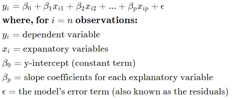
The formula of the linear regression doesn't change, it remains y= m*X+b, only the number of coefficients increases
Advantages/Features of Multiple Linear Regression
- The chances of getting a better-fit increase as the generated models are dependent on more than 1 feature
- Multiple Linear Regression can detect outliers and anomalies very effectively.
Disadvantages/Shortcomings of Multiple Linear Regression
- The problem of overfitting is very prevalent here, as we can use all features to generate the model, so the model can start "memorizing" the values
- Accuracy decreases as the linearity of the dataset decreases.
Multiple Linear Regression
Multiple linear regression (MLR) or multiple regression, is a statistical technique that uses several preparatory variables to predict the outcome of a response variable. The goal of multiple linear regression (MLR) is to model the linear relationship between the explanatory (independent) variables and response (dependent) variable.
In essence, multiple regression is the extension of ordinary least-squares (OLS) regression that involves more than one explanatory variable.
Simple linear regression is a method that allows an analyst or statistician to make predictions about one variable based on the information that is known about another variable. Linear regression can only be used when one has two continuous variables—an independent variable and a dependent variable. The independent variable is the parameter that is used to calculate the dependent variable or outcome. A multiple regression model extends to several explanatory variables.
The multiple regression model is based on the following assumptions:
- Linearity: There is a linear relationship between the dependent variables and the independent variables.
- Correlation: The independent variables are not too highly correlated with each other.
- yi observations are selected independently and randomly from the population.
- Normal Distribution: Residuals should be normally distributed with a mean of 0 and variance σ.
Multiple Linear Regression Example
Let's take the example of the IRIS dataset, you can directly import it from the sklearn dataset repository. Feel free to use any dataset, there some very good datasets available on kaggle and with Google Colab.
Before we start with this, it is highly recommended you read the following tutorials
1. Using SkLearn
- from pandas import DataFrame
- from sklearn import linear_model
- import statsmodels.api as sm
- Stock_Market = {'Year': [2017,2017,2017,2017,2017,2017,2017,2017,2017,2017,2017,2017,2016,2016,2016,2016,2016,2016,2016,2016,2016,2016,2016,2016],
- 'Month': [12, 11,10,9,8,7,6,5,4,3,2,1,12,11,10,9,8,7,6,5,4,3,2,1],
- 'Interest_Rate': [2.75,2.5,2.5,2.5,2.5,2.5,2.5,2.25,2.25,2.25,2,2,2,1.75,1.75,1.75,1.75,1.75,1.75,1.75,1.75,1.75,1.75,1.75],
- 'Unemployment_Rate': [5.3,5.3,5.3,5.3,5.4,5.6,5.5,5.5,5.5,5.6,5.7,5.9,6,5.9,5.8,6.1,6.2,6.1,6.1,6.1,5.9,6.2,6.2,6.1],
- 'Stock_Index_Price': [1464,1394,1357,1293,1256,1254,1234,1195,1159,1167,1130,1075,1047,965,943,958,971,949,884,866,876,822,704,719]
- }
- df = DataFrame(Stock_Market,columns=['Year','Month','Interest_Rate','Unemployment_Rate','Stock_Index_Price'])
- X = df[['Interest_Rate','Unemployment_Rate']]
- Y = df['Stock_Index_Price']
- regr = linear_model.LinearRegression()
- regr.fit(X, Y)
- print('Intercept: \n', regr.intercept_) Multiple Linear Regression using Python
- print('Coefficients: \n', regr.coef_)
the output that I am getting is :
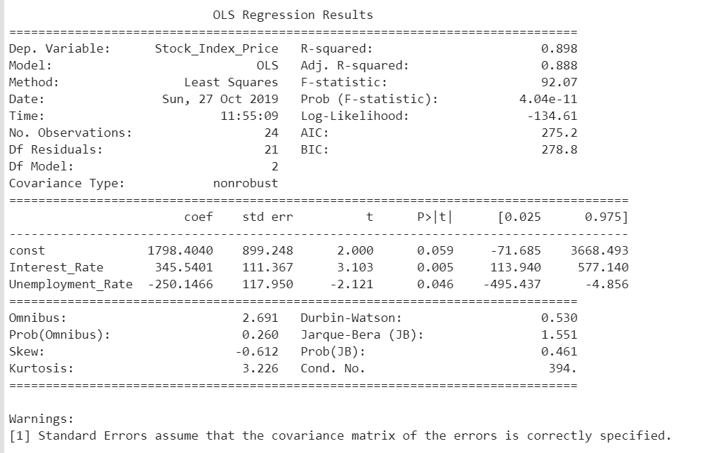
Intercept: 1798.4039776258546
Coefficients: [ 345.54008701 -250.14657137]
- # prediction with sklearn
- New_Interest_Rate = 2.75
- New_Unemployment_Rate = 5.3
- print ('Predicted Stock Index Price: \n', regr.predict([[New_Interest_Rate ,New_Unemployment_Rate]]))
MLR_SkLearn.py
- from pandas import DataFrame
- from sklearn import linear_model
- import statsmodels.api as sm
- Stock_Market = {'Year': [2017,2017,2017,2017,2017,2017,2017,2017,2017,2017,2017,2017,2016,2016,2016,2016,2016,2016,2016,2016,2016,2016,2016,2016],
- 'Month': [12, 11,10,9,8,7,6,5,4,3,2,1,12,11,10,9,8,7,6,5,4,3,2,1],
- 'Interest_Rate': [2.75,2.5,2.5,2.5,2.5,2.5,2.5,2.25,2.25,2.25,2,2,2,1.75,1.75,1.75,1.75,1.75,1.75,1.75,1.75,1.75,1.75,1.75],
- 'Unemployment_Rate': [5.3,5.3,5.3,5.3,5.4,5.6,5.5,5.5,5.5,5.6,5.7,5.9,6,5.9,5.8,6.1,6.2,6.1,6.1,6.1,5.9,6.2,6.2,6.1],
- 'Stock_Index_Price': [1464,1394,1357,1293,1256,1254,1234,1195,1159,1167,1130,1075,1047,965,943,958,971,949,884,866,876,822,704,719]
- }
- df = DataFrame(Stock_Market,columns=['Year','Month','Interest_Rate','Unemployment_Rate','Stock_Index_Price'])
- X = df[['Interest_Rate','Unemployment_Rate']] # here we have 2 variables for multiple regression. If you just want to use one variable for simple linear regression, then use X = df['Interest_Rate'] for example.Alternatively, you may add additional variables within the brackets
- Y = df['Stock_Index_Price']
- # with sklearn
- regr = linear_model.LinearRegression()
- regr.fit(X, Y)
- print('Intercept: \n', regr.intercept_)
- print('Coefficients: \n', regr.coef_)
- # prediction with sklearn
- New_Interest_Rate = 2.75
- New_Unemployment_Rate = 5.3
- print ('Predicted Stock Index Price: \n', regr.predict([[New_Interest_Rate ,New_Unemployment_Rate]]))
Intercept: 1798.4039776258546
Coefficients: [ 345.54008701 -250.14657137]
Predicted Stock Index Price: [1422.86238865]
- print_model = model.summary()
- print(print_model)
2. Using NumPy
- import numpy as np
- import pandas as pd
- import matplotlib.pyplot as plt
- import seaborn as sns
- my_data = pd.read_csv('home.txt',names=["size","bedroom","price"])
- #we need to normalize the features using mean normalization
- my_data = (my_data - my_data.mean())/my_data.std()
- #setting the matrixes
- X = my_data.iloc[:,0:2]
- ones = np.ones([X.shape[0],1])
- X = np.concatenate((ones,X),axis=1)
- y = my_data.iloc[:,2:3].values #.values converts it from pandas.core.frame.DataFrame to numpy.ndarray
- theta = np.zeros([1,3])
- sns.heatmap(X)

- def computeCost(X,y,theta):
- tobesummed = np.power(((X @ theta.T)-y),2)
- return np.sum(tobesummed)/(2 * len(X))
- def gradientDescent(X,y,theta,iters,alpha):
- cost = np.zeros(iters)
- for i in range(iters):
- theta = theta - (alpha/len(X)) * np.sum(X * (X @ theta.T - y), axis=0)
- cost[i] = computeCost(X, y, theta)
- return theta,cost
- #set hyperparameters
- alpha = 0.01
- iters = 1000
- g,cost = gradientDescent(X,y,theta,iters,alpha)
- print(g)
- finalCost = computeCost(X,y,g)
- print(finalCost)
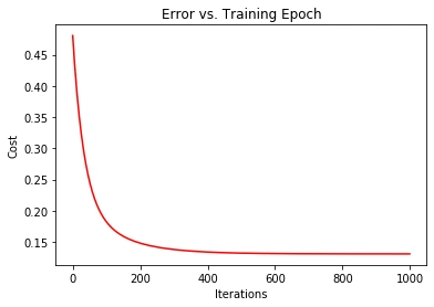
The output that I am getting is
[[-1.10868761e-16 8.78503652e-01 -4.69166570e-02]] 0.13070336960771892
- fig, ax = plt.subplots()
- ax.plot(np.arange(iters), cost, 'r')
- ax.set_xlabel('Iterations')
- ax.set_ylabel('Cost')
- ax.set_title('Error vs. Training Epoch')
MLR_NumPy.py
- import numpy as np
- import pandas as pd
- import matplotlib.pyplot as plt
- import seaborn as sns
- my_data = pd.read_csv('home.txt',names=["size","bedroom","price"])
- #we need to normalize the features using mean normalization
- my_data = (my_data - my_data.mean())/my_data.std()
- #setting the matrixes
- X = my_data.iloc[:,0:2]
- ones = np.ones([X.shape[0],1])
- X = np.concatenate((ones,X),axis=1)
- y = my_data.iloc[:,2:3].values #.values converts it from pandas.core.frame.DataFrame to numpy.ndarray
- theta = np.zeros([1,3])
- sns.heatmap(X)
- #computecost
- def computeCost(X,y,theta):
- tobesummed = np.power(((X @ theta.T)-y),2)
- return np.sum(tobesummed)/(2 * len(X))
- def gradientDescent(X,y,theta,iters,alpha):
- cost = np.zeros(iters)
- for i in range(iters):
- theta = theta - (alpha/len(X)) * np.sum(X * (X @ theta.T - y), axis=0)
- cost[i] = computeCost(X, y, theta)
- return theta,cost
- #set hyper parameters
- alpha = 0.01
- iters = 1000
- g,cost = gradientDescent(X,y,theta,iters,alpha)
- print(g)
- finalCost = computeCost(X,y,g)
- print(finalCost)
- fig, ax = plt.subplots()
- ax.plot(np.arange(iters), cost, 'r')
- ax.set_xlabel('Iterations')
- ax.set_ylabel('Cost')
- ax.set_title('Error vs. Training Epoch')
- import matplotlib.pyplot as plt
- import tensorflow as tf
- import tensorflow.contrib.learn as skflow
- from sklearn.utils import shuffle
- import numpy as np
- import pandas as pd
- import seaborn as sns
- df = pd.read_csv("boston.csv", header=0)
- print (df.describe())
- sns.heatmap(df)

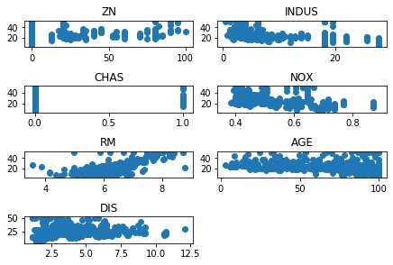
- f, ax1 = plt.subplots()
- y = df['MEDV']
- for i in range (1,8):
- number = 420 + i
- ax1.locator_params(nbins=3)
- ax1 = plt.subplot(number)
- plt.title(list(df)[i])
- ax1.scatter(df[df.columns[i]],y) #Plot a scatter draw of the datapoints
- plt.tight_layout(pad=0.4, w_pad=0.5, h_pad=1.0)
- plt.show()
- X = tf.placeholder("float", name="X") # create symbolic variables
- Y = tf.placeholder("float", name = "Y")
- with tf.name_scope("Model"):
- w = tf.Variable(tf.random_normal([2], stddev=0.01), name="b0") # create a shared variable
- b = tf.Variable(tf.random_normal([2], stddev=0.01), name="b1") # create a shared variable
- def model(X, w, b):
- return tf.multiply(X, w) + b # We just define the line as X*w + b0
- y_model = model(X, w, b)
- with tf.name_scope("CostFunction"):
- cost = tf.reduce_mean(tf.pow(Y-y_model, 2)) # use sqr error for cost function
- train_op = tf.train.AdamOptimizer(0.001).minimize(cost)
- sess = tf.Session()
- init = tf.initialize_all_variables()
- tf.train.write_graph(sess.graph, '/home/bonnin/linear2','graph.pbtxt')
- cost_op = tf.summary.scalar("loss", cost)
- merged = tf.summary.merge_all()
- sess.run(init)
- writer = tf.summary.FileWriter('/home/bonnin/linear2', sess.graph)
- xvalues = df[[df.columns[2], df.columns[4]]].values.astype(float)
- yvalues = df[df.columns[12]].values.astype(float)
- b0temp=b.eval(session=sess)
- b1temp=w.eval(session=sess)
- for a in range (1,50):
- cost1=0.0
- for i, j in zip(xvalues, yvalues):
- sess.run(train_op, feed_dict={X: i, Y: j})
- cost1+=sess.run(cost, feed_dict={X: i, Y: i})/506.00
- xvalues, yvalues = shuffle (xvalues, yvalues)
- print ("Cost over iterations",cost1)
- b0temp=b.eval(session=sess)
- b1temp=w.eval(session=sess)
- print("the final equation comes out to be", b0temp,"+",b1temp,"*X","\n Cost :",cost1)
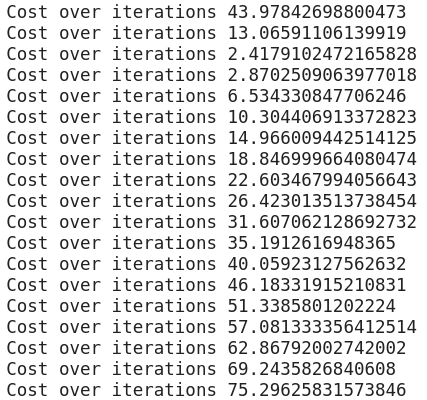
The output that I am getting is
the final equation comes out to be [4.7545404 7.7991614] + [1.0045488 7.807921 ] *X
Cost: 75.29625831573846
MLR_TensorFlow.py
- import tensorflow as tf
- import tensorflow.contrib.learn as skflow
- from sklearn.utils import shuffle
- import numpy as np
- import pandas as pd
- df = pd.read_csv("boston.csv", header=0)
- print (df.describe())
- f, ax1 = plt.subplots()
- import seaborn as sns
- sns.heatmap(df)
- y = df['MEDV']
- for i in range (1,8):
- number = 420 + i
- ax1.locator_params(nbins=3)
- ax1 = plt.subplot(number)
- plt.title(list(df)[i])
- ax1.scatter(df[df.columns[i]],y) #Plot a scatter draw of the datapoints
- plt.tight_layout(pad=0.4, w_pad=0.5, h_pad=1.0)
- plt.show()
- X = tf.placeholder("float", name="X") # create symbolic variables
- Y = tf.placeholder("float", name = "Y")
- with tf.name_scope("Model"):
- w = tf.Variable(tf.random_normal([2], stddev=0.01), name="b0") # create a shared variable
- b = tf.Variable(tf.random_normal([2], stddev=0.01), name="b1") # create a shared variable
- def model(X, w, b):
- return tf.multiply(X, w) + b # We just define the line as X*w + b0
- y_model = model(X, w, b)
- with tf.name_scope("CostFunction"):
- cost = tf.reduce_mean(tf.pow(Y-y_model, 2)) # use sqr error for cost function
- train_op = tf.train.AdamOptimizer(0.001).minimize(cost)
- sess = tf.Session()
- init = tf.initialize_all_variables()
- tf.train.write_graph(sess.graph, '/home/bonnin/linear2','graph.pbtxt')
- cost_op = tf.summary.scalar("loss", cost)
- merged = tf.summary.merge_all()
- sess.run(init)
- writer = tf.summary.FileWriter('/home/bonnin/linear2', sess.graph)
- xvalues = df[[df.columns[2], df.columns[4]]].values.astype(float)
- yvalues = df[df.columns[12]].values.astype(float)
- b0temp=b.eval(session=sess)
- b1temp=w.eval(session=sess)
- for a in range (1,50):
- cost1=0.0
- for i, j in zip(xvalues, yvalues):
- sess.run(train_op, feed_dict={X: i, Y: j})
- cost1+=sess.run(cost, feed_dict={X: i, Y: i})/506.00
- xvalues, yvalues = shuffle (xvalues, yvalues)
- print ("Cost over iterations",cost1)
- b0temp=b.eval(session=sess)
- b1temp=w.eval(session=sess)
- print("the final equation comes out to be", b0temp,"+",b1temp,"*X")
Conclusion
In this article, we studied what is regression, types of regression and why should we use multiple linear regression, how do we calculate multiple linear regression, advantages of multiple linear regression, disadvantages of multiple linear regression, multiple linear regression example using sklearn, numpy, and TensorFlow. Hope you were able to understand each and everything. For any doubts, please comment on your query.
In the next article, we will learn about the Decision Tree.
Congratulations!!! You have climbed your next step in becoming a successful ML Engineer.
Next Article In this Series >> Decision Tree
tushar kshirsagarPosted Aug 26, 2021, 4:16 PM
What is model here? no clue what object it carries print_model = model.summary() print(print_model)
Sourav Kumar DasPosted Nov 11, 2019, 5:15 AM
Nice Superb useful article Sir.