Logistic Regression using Python

In the previous article, we studied Linear Regression. One thing that I believe is that if we can correlate anything with us or our life, there are greater chances of understanding the concept. So I will try to explain everything by relating it to humans.

What is Regression? Types of Regression

For reading about the regression, please read the article Linear Regression

What is Logistic Regression?

Logistic regression is the appropriate regression analysis to conduct when the dependent variable is dichotomous (binary). Like all regression analyses, logistic regression is a predictive analysis. Logistic regression is used to describe data and to explain the relationship between one dependent binary variable and one or more nominal, ordinal, interval or ratio-level independent variables. Logistic regression models the probabilities for classification problems with two possible outcomes. It’s an extension of the linear regression model for classification problems.

What is it used for?

Logistic regression is used to describe data and to explain the relationship between one dependent binary variable and one or more nominal, ordinal, interval or ratio-level independent variables.

Difference between Linear and Logistic Regression

BASIS FOR COMPARISON	LINEAR REGRESSION	LOGISTIC REGRESSION
Basic	The data is modeled using a straight line.	The probability of some obtained event is represented as a linear function of a combination of predictor variables.
Linear relationship between the dependent and independent variables	Is required	Not required
The independent variable	Could be correlated with each other. (Especially in multiple linear regression)	Should not be correlated with each other (no multicollinearity exists).
Outcome	the outcome (dependent variable) is continuous. It can have any one of an infinite number of possible values.	the outcome (dependent variable) has only a limited number of possible values.
Dependent Variable	Linear regression is used when your response variable is continuous. For instance, weight, height, number of hours, etc.	Logistic regression is used when the response variable is categorical in nature. For instance, yes/no, true/false, red/green/blue, 1st/2nd/3rd/4th, etc.
Equation	Linear regression gives an equation that is of the form Y = MX + C, which means equation with degree 1.	logistic regression gives an equation which is of the form Y = e^X + e^-X
Coefficient Interpretation	the coefficient interpretation of independent variables is quite straightforward (i.e. holding all other variables constant, with a unit increase in this variable, the dependent variable is expected to increase/decrease by xxx).	depends on the family (binomial, Poisson, etc.) and link (log, logit, inverse-log, etc.) you use, the interpretation is different.
Error Minimization Technique	uses ordinary least squares method to minimize the errors and arrive at a best possible fit	uses a maximum likelihood method to arrive at the solution.

Why is Logistic Regression called so?

The meaning of the term regression is very simple: any process that attempts to find relationships between variables is called regression. Logistic regression is a regression because it finds relationships between variables. It is logistic because it uses a logistic function as a link function. Hence the full name.

What is the goal of Logistic Regression?

The goal of logistic regression is to correctly predict the category of outcome for individual cases using the most parsimonious model. To accomplish this goal, a model is created that includes all predictor variables that are useful in predicting the response variable. In other words, The goal of logistic regression is to find the best fitting (yet biologically reasonable) model to describe the relationship between the dichotomous characteristic of interest (dependent variable = response or outcome variable) and a set of independent (predictor or explanatory) variables.

Advantages/Features of Logistic Regression

1. Logistic Regression performs well when the dataset is linearly separable.

2. Logistic regression is less prone to over-fitting but it can overfit in high dimensional datasets. You should consider Regularization (L1 and L2) techniques to avoid over-fitting in these scenarios.

3. Logistic Regression not only gives a measure of how relevant a predictor (coefficient size) is, but also its direction of association (positive or negative).

4. Logistic regression is easier to implement, interpret, and very efficient to train.

Disadvantages/Shortcomings of Logistic Regression

1. The main limitation of Logistic Regression is the assumption of linearity between the dependent variable and the independent variables. In the real world, the data is rarely linearly separable. Most of the time data would be a jumbled mess.
2. If the number of observations is lesser than the number of features, Logistic Regression should not be used, otherwise, it may lead to overfitting.
3. Logistic Regression can only be used to predict discrete functions. Therefore, the dependent variable of Logistic Regression is restricted to the discrete number set. This restriction itself is problematic, as it is prohibitive to the prediction of continuous data.

Types of Logistic Regression

1. Binary Logistic Regression

The categorical response has only two 2 possible outcomes. Example: Spam or Not

2. Multinomial Logistic Regression

Three or more categories without ordering. Example: Predicting which food is preferred more (Veg, Non-Veg, Vegan)

3. Ordinal Logistic Regression

Three or more categories with ordering. Example: Movie rating from 1 to 5

Key Terms

For reading about the basic terms of regression, please read the article Linear Regression

1. Logit

In statistics, the logit function or the log-odds is the logarithm of the odds p/(1 − p) where p is the probability. It is a type of function that creates a map of probability values from [0,1] to $(-\infty ,+\infty )$ It is the inverse of the sigmoidal "logistic" function or logistic transform used in mathematics, especially in statistics.

In deep learning, the term logits layer is popularly used for the last neuron layer of neural networks used for classification tasks, which produce raw prediction values as real numbers ranging from $(-\infty ,+\infty )$ .

2. Logistic Function

The logistic function is a sigmoid function, which takes any real input t, ( $t\in \mathbb {R}$ ), and outputs a value between zero and one; for the logit, this is interpreted as taking input log-odds and having output probability. The standard logistic function $\sigma :\mathbb {R} \rightarrow (0,1)$ is defined as follows:

$\sigma (t)={\frac {e^{t}}{e^{t}+1}}={\frac {1}{1+e^{-t}}}$

3. Inverse of Logistic Function

We can now define the logit (log odds) function as the inverse $g=\sigma ^{-1}$ of the standard logistic function. It is easy to see that it satisfies:

$g(p(x))=\sigma ^{-1}(p(x))=\operatorname {logit} p(x)=\ln \left({\frac {p(x)}{1-p(x)}}\right)=\beta _{0}+\beta _{1}x,$

and equivalently, after exponentiating both sides we have the odds:

where,

g is the logit function. The equation for g(p(x)) illustrates that the logit (i.e., log-odds or natural logarithm of the odds) is equivalent to the linear regression expression.
ln denotes the natural logarithm.
The formula for p(x) illustrates that the probability of the dependent variable for a given case is equal to the value of the logistic function of the linear regression expression. This is important as it shows that the value of the linear regression expression can vary from negative to positive infinity and yet, after transformation, the resulting probability p(x) ranges between 0 and 1.
$\beta _{0}$ is the intercept from the linear regression equation (the value of the criterion when the predictor is equal to zero).
$\beta _{1}x$ is the regression coefficient multiplied by some value of the predictor.
base 'e' denotes the exponential function.

4. Odds

The odds of the dependent variable equaling a case (given some linear combination x of the predictors) is equivalent to the exponential function of the linear regression expression. This illustrates how the logit serves as a link function between the probability and the linear regression expression. Given that the logit ranges between negative and positive infinity, it provides an adequate criterion upon which to conduct linear regression and the logit is easily converted back into the odds.

So we define odds of the dependent variable equaling a case (given some linear combination x of the predictors) as follows:

${\text{odds}}=e^{\beta _{0}+\beta _{1}x}.$

5. Odds Ration

For a continuous independent variable, the odds ratio can be defined as:

$\mathrm {OR} ={\frac {\operatorname {odds} (x+1)}{\operatorname {odds} (x)}}={\frac {\left({\frac {F(x+1)}{1-F(x+1)}}\right)}{\left({\frac {F(x)}{1-F(x)}}\right)}}={\frac {e^{\beta _{0}+\beta _{1}(x+1)}}{e^{\beta _{0}+\beta _{1}x}}}=e^{\beta _{1}}$

This exponential relationship provides an interpretation for $\beta _{1}$ : The odds multiply by $e^{\beta _{1}}$ for every 1-unit increase in x.

For a binary independent variable, the odds ratio is defined as ${\frac {ad}{bc}}$ where a, b, c, and d are cells in a 2×2 contingency table.

6. Multiple Explanatory Variable

If there are multiple explanatory variables, the above expression can be revised to

$\beta _{0}+\beta _{1}x_{1}+\beta _{2}x_{2}+\cdots +\beta _{m}x_{m}=\beta _{0}+\sum _{i=1}^{m}\beta _{i}x_{i}$

Then when this is used in the equation relating the log odds of success to the values of the predictors, the linear regression will be a multiple regression with m explanators; the parameters $\beta _{j}$ for all j = 0, 1, 2, ..., m are all estimated.

Again, the more traditional equations are:

$\log {\frac {p}{1-p}}=\beta _{0}+\beta _{1}x_{1}+\beta _{2}x_{2}+\cdots +\beta _{m}x_{m}$

and

$p={\frac {1}{1+b^{-(\beta _{0}+\beta _{1}x_{1}+\beta _{2}x_{2}+\cdots +\beta _{m}x_{m})}}}$

where usually b = e.

Logistic Regression

logistic regression produces a logistic curve, which is limited to values between 0 and 1. Logistic regression is similar to linear regression, but the curve is constructed using the natural logarithm of the “odds” of the target variable, rather than the probability. Moreover, the predictors do not have to be normally distributed or have equal variance in each group.

The logistic Regression Equation is given by

$\displaystyle \frac {p}{1-p} = e^{b_0+b_1*x}$

Taking natural log on both sides we get

$\displaystyle \ln{\frac {p}{1-p}} = b_0+b_1*x$

Till now, we have seen the equation for one variable, so now following is the equation when the number of variables is more than one

$p={\frac {1}{1+b^{-(\beta _{0}+\beta _{1}x_{1}+\beta _{2}x_{2}+\cdots +\beta _{m}x_{m})}}}$

where usually b = e. OR

$\log {\frac {p}{1-p}}=\beta _{0}+\beta _{1}x_{1}+\beta _{2}x_{2}+\cdots +\beta _{m}x_{m}$

Let me use an example, to explain in which cases we will use logistic Regression:

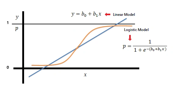
Linear regression will fail in cases where the boundaries are pre-defined, as if we use Linear Regression, it may predict outside the boundaries. For example, let's take the example of housing price prediction, that we used in the last article, so when predicting, there are chances that linear regression would predict the price too high, which may not be practically possible, or too loss such as may be negative.

Since in the case of binary classification, there are only two possible outcomes, but it is not necessary that the input data be distributed uniformly, it is often seen that the class '0' data point if found in the decision boundary of class '1'. Since, the sigmoid function is a curve, the possibility of getting a perfect fit increases, hence resolving the problem of having

Logistic Regression Example

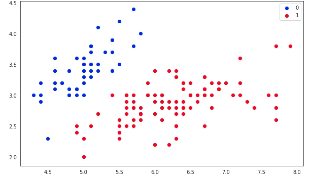
Let's take the example of the IRIS dataset, you can directly import it from the sklearn dataset repository. Feel free to use any dataset, there some very good datasets available on kaggle and with Google Colab.

Before we start with this, it is highly recommended you read the following tutorials

1. Using SKLearn

%matplotlib inline
import numpy as np
import matplotlib.pyplot as plt
import seaborn as sns
from sklearn import datasets
from sklearn.linear_model import LogisticRegression

In the above code, we are importing the required libraries, that we will be using.

iris = datasets.load_iris()

Loading the IRIS dataset from the sklearn dataset repository

X = iris.data[:, :2]
y = (iris.target != 0) * 1

Manipulating and pre-processing the data, so that it can be fed to the model.

plt.figure(figsize=(10, 6))
plt.scatter(X[y == 0][:, 0], X[y == 0][:, 1], color='b', label='0')
plt.scatter(X[y == 1][:, 0], X[y == 1][:, 1], color='r', label='1')
plt.legend();

Let us try to visualize the imported data

model = LogisticRegression(C=1e2)
%time model.fit(X, y)
print(model.intercept_, model.coef_,model.n_iter_)

In the above code, we are timing the training process using the "%time", and then printing the model parameters.

The output that I got for training is:

CPU times: user 2.45 ms, sys: 1.06 ms, total: 3.51 ms Wall time: 1.76 ms

model.itercept: [-33.08987216]

model.coeffiecent: [[ 14.75218964 -14.87575477]]

number of iterations: [12]

plt.figure(figsize=(10, 6))
plt.scatter(X[y == 0][:, 0], X[y == 0][:, 1], color='b', label='0')
plt.scatter(X[y == 1][:, 0], X[y == 1][:, 1], color='r', label='1')
plt.legend()
x1_min, x1_max = X[:,0].min(), X[:,0].max(),
x2_min, x2_max = X[:,1].min(), X[:,1].max(),
xx1, xx2 = np.meshgrid(np.linspace(x1_min, x1_max), np.linspace(x2_min, x2_max))
grid = np.c_[xx1.ravel(), xx2.ravel()]
probs = model.predict(grid).reshape(xx1.shape)
plt.contour(xx1, xx2, probs, [0.5], linewidths=1, colors='black');

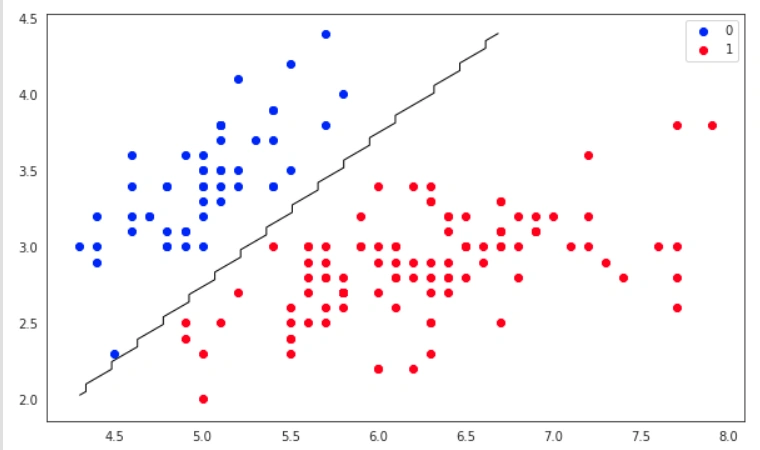
The above code, lets us visulaize the regression line with respect to the input data.

pred = model.predict(X[1:2])
print(pred)

In the above code, we predict that the class of the sample X[1:2], and the class result out to be [0], which is correct

LR_Sklearn.py

%matplotlib inline
import numpy as np
import matplotlib.pyplot as plt
import seaborn as sns
from sklearn import datasets
from sklearn.linear_model import LogisticRegression
iris = datasets.load_iris()
X = iris.data[:, :2]
y = (iris.target != 0) * 1
plt.figure(figsize=(10, 6))
plt.scatter(X[y == 0][:, 0], X[y == 0][:, 1], color='b', label='0')
plt.scatter(X[y == 1][:, 0], X[y == 1][:, 1], color='r', label='1')
plt.legend();
model = LogisticRegression(C=1e2)
%time model.fit(X, y)
print(model.intercept_, model.coef_,model.n_iter_)
plt.figure(figsize=(10, 6))
plt.scatter(X[y == 0][:, 0], X[y == 0][:, 1], color='b', label='0')
plt.scatter(X[y == 1][:, 0], X[y == 1][:, 1], color='r', label='1')
plt.legend()
x1_min, x1_max = X[:,0].min(), X[:,0].max(),
x2_min, x2_max = X[:,1].min(), X[:,1].max(),
xx1, xx2 = np.meshgrid(np.linspace(x1_min, x1_max), np.linspace(x2_min, x2_max))
grid = np.c_[xx1.ravel(), xx2.ravel()]
probs = model.predict(grid).reshape(xx1.shape)
plt.contour(xx1, xx2, probs, [0.5], linewidths=1, colors='black');

2. Using Numpy

%matplotlib inline
import numpy as np
import matplotlib.pyplot as plt
import seaborn as sns
from sklearn import datasets a

In the above code, we are importing the required libraries, that we will be using.

iris = datasets.load_iris()

Loading the IRIS dataset from the sklearn dataset repository

X = iris.data[:, :2]
y = (iris.target != 0) * 1

Manipulating and pre-processing the data, so that it can be fed to the model.

plt.figure(figsize=(10, 6))
plt.scatter(X[y == 0][:, 0], X[y == 0][:, 1], color='b', label='0')
plt.scatter(X[y == 1][:, 0], X[y == 1][:, 1], color='r', label='1')
plt.legend();

Let us try to visualize the imported data

class LogisticRegression:
def __init__(self, lr=0.01, num_iter=100000, fit_intercept=True, verbose=False):
self.lr = lr
self.num_iter = num_iter
self.fit_intercept = fit_intercept
self.verbose = verbose
def __add_intercept(self, X):
intercept = np.ones((X.shape[0], 1))
return np.concatenate((intercept, X), axis=1)
def __sigmoid(self, z):
return 1 / (1 + np.exp(-z))
def __loss(self, h, y):
return (-y * np.log(h) - (1 - y) * np.log(1 - h)).mean()
def fit(self, X, y):
if self.fit_intercept:
X = self.__add_intercept(X)
# weights initialization
self.theta = np.zeros(X.shape[1])
for i in range(self.num_iter):
z = np.dot(X, self.theta)
h = self.__sigmoid(z)
gradient = np.dot(X.T, (h - y)) / y.size
self.theta -= self.lr * gradient
z = np.dot(X, self.theta)
h = self.__sigmoid(z)
loss = self.__loss(h, y)
if(self.verbose ==True and i % 10000 == 0):
print(f'loss: {loss} \t')
def predict_prob(self, X):
if self.fit_intercept:
X = self.__add_intercept(X)
return self.__sigmoid(np.dot(X, self.theta))
def predict(self, X):
return self.predict_prob(X).round()

In the above code, we created a user-defined class "LogisticRegression", which contain all the methods required to result out the desired regression line

__init__ - constructor to initialize all the required variables with default values or initial values
__add_intercept - to find the model intercept value
__sigmoid - function to return sigmoid curve
__loss - function to return loss
fit - function to calculate and return the regression line
predict_prob - helper function used for prediction
predict - function to return predicted value

model = LogisticRegression(lr=0.1, num_iter=3000)
%time model.fit(X, y)

In the above code, we intiantiate the LogisticRegression class, and then provide 'X' and 'y' as the parameters to the fit function to result out the desired regression line

preds = model.predict(X[1:2])
print(preds)

In the above code, we ask the model to tell the class to which our sample X[1:2] belong and the result that we get is [0.], which is correte

print(model.theta)

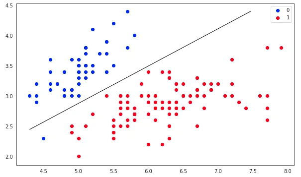
Now we print the parameter values of the resulted model.

Parameter values of my model are :

[-1.44894305 4.25546329 -6.89489245]

plt.figure(figsize=(10, 6))
plt.scatter(X[y == 0][:, 0], X[y == 0][:, 1], color='b', label='0')
plt.scatter(X[y == 1][:, 0], X[y == 1][:, 1], color='r', label='1')
plt.legend()
x1_min, x1_max = X[:,0].min(), X[:,0].max(),
x2_min, x2_max = X[:,1].min(), X[:,1].max(),
xx1, xx2 = np.meshgrid(np.linspace(x1_min, x1_max), np.linspace(x2_min, x2_max))
grid = np.c_[xx1.ravel(), xx2.ravel()]
probs = model.predict_prob(grid).reshape(xx1.shape)
plt.contour(xx1, xx2, probs, [0.5], linewidths=1, colors='black');

The above code, will provide us a visualization of the generated regression line with respect to the input data.

LR_NumPy.py

%matplotlib inline
import numpy as np
import matplotlib.pyplot as plt
import seaborn as sns
from sklearn import datasets
iris = datasets.load_iris()
X = iris.data[:, :2]
y = (iris.target != 0) * 1
plt.figure(figsize=(10, 6))
plt.scatter(X[y == 0][:, 0], X[y == 0][:, 1], color='b', label='0')
plt.scatter(X[y == 1][:, 0], X[y == 1][:, 1], color='r', label='1')
plt.legend();
class LogisticRegression:
def __init__(self, lr=0.01, num_iter=100000, fit_intercept=True, verbose=False):
self.lr = lr
self.num_iter = num_iter
self.fit_intercept = fit_intercept
self.verbose = verbose
def __add_intercept(self, X):
intercept = np.ones((X.shape[0], 1))
return np.concatenate((intercept, X), axis=1)
def __sigmoid(self, z):
return 1 / (1 + np.exp(-z))
def __loss(self, h, y):
return (-y * np.log(h) - (1 - y) * np.log(1 - h)).mean()
def fit(self, X, y):
if self.fit_intercept:
X = self.__add_intercept(X)
# weights initialization
self.theta = np.zeros(X.shape[1])
for i in range(self.num_iter):
z = np.dot(X, self.theta)
h = self.__sigmoid(z)
gradient = np.dot(X.T, (h - y)) / y.size
self.theta -= self.lr * gradient
z = np.dot(X, self.theta)
h = self.__sigmoid(z)
loss = self.__loss(h, y)
if(self.verbose ==True and i % 10000 == 0):
print(f'loss: {loss} \t')
def predict_prob(self, X):
if self.fit_intercept:
X = self.__add_intercept(X)
return self.__sigmoid(np.dot(X, self.theta))
def predict(self, X):
return self.predict_prob(X).round()
model = LogisticRegression(lr=0.1, num_iter=3000)
%time model.fit(X, y)
preds = model.predict(X[1:2])
print(preds)
print(model.theta)
plt.figure(figsize=(10, 6))
plt.scatter(X[y == 0][:, 0], X[y == 0][:, 1], color='b', label='0')
plt.scatter(X[y == 1][:, 0], X[y == 1][:, 1], color='r', label='1')
plt.legend()
x1_min, x1_max = X[:,0].min(), X[:,0].max(),
x2_min, x2_max = X[:,1].min(), X[:,1].max(),
xx1, xx2 = np.meshgrid(np.linspace(x1_min, x1_max), np.linspace(x2_min, x2_max))
grid = np.c_[xx1.ravel(), xx2.ravel()]
probs = model.predict_prob(grid).reshape(xx1.shape)
plt.contour(xx1, xx2, probs, [0.5], linewidths=1, colors='black');

3. Using TensorFlow

from __future__ import print_function
import tensorflow as tf

In the above code, we are importing the required libraries

# Import MNIST data
from tensorflow.examples.tutorials.mnist import input_data
mnist = input_data.read_data_sets("/tmp/data/", one_hot=True)

Using the TensorFlow's dataset library, we are importing MNIST dataset

# Parameters
learning_rate = 0.01
training_epochs = 100
batch_size = 100
display_step = 50

In the above code, we are assigning the values to all the global parameters.

# tf Graph Input
x = tf.placeholder(tf.float32, [None, 784]) # mnist data image of shape 28*28=784
y = tf.placeholder(tf.float32, [None, 10]) # 0-9 digits recognition => 10 classes
# Set model weights
W = tf.Variable(tf.zeros([784, 10]))
b = tf.Variable(tf.zeros([10]))

Here we are setting X and Y as the actual training data and the W and b as the trainable data, where:

W means Weight
b means bais
X means the dependent variable
Y means the independent variable

# Construct model
pred = tf.nn.softmax(tf.matmul(x, W) + b) # Softmax
# Minimize error using cross entropy
cost = tf.reduce_mean(-tf.reduce_sum(y*tf.log(pred), reduction_indices=1))
# Gradient Descent
optimizer = tf.train.GradientDescentOptimizer(learning_rate).minimize(cost)
# Initialize the variables (i.e. assign their default value)
init = tf.global_variables_initializer()

In the above code, we are

setting the model using the Softmax method
cost calculation will be based on the reduced mean method
the optimizer is chosen to be Gradient Descent which minimizes cost
the variable initializer is chosen to be a global variable initializer

# Start training
with tf.Session() as sess:
# Run the initializer
sess.run(init)
# Training cycle
for epoch in range(training_epochs):
avg_cost = 0.
total_batch = int(mnist.train.num_examples/batch_size)
# Loop over all batches
for i in range(total_batch):
batch_xs, batch_ys = mnist.train.next_batch(batch_size)
# Run optimization op (backprop) and cost op (to get loss value)
_, c = sess.run([optimizer, cost], feed_dict={x: batch_xs,
y: batch_ys})
# Compute average loss
avg_cost += c / total_batch
# Display logs per epoch step
if (epoch+1) % display_step == 0:
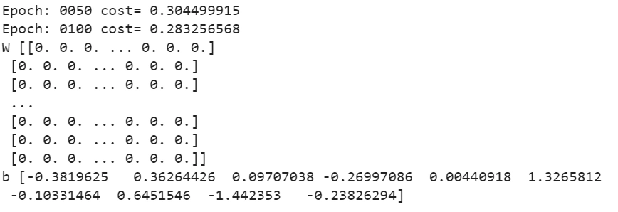
print("Epoch:", '%04d' % (epoch+1), "cost=", "{:.9f}".format(avg_cost))
training_cost = sess.run(cost, feed_dict ={x: batch_xs,
y: batch_ys})
weight = sess.run(W)
bias = sess.run(b)

In the above code, we start training and cost is printed after every 50 epochs. Here since the number of data points are large and processing in one go may cause crashes, so we train in batches.

print("W",weight,"\nb",bias)
eq= tf.math.sigmoid((tf.matmul(x, weight) + bias))

In the above code, we print the weight and bias of the learned model and then form the Logistic Regression Equation.

LR_tensorflow.py

from __future__ import print_function
import tensorflow as tf
# Import MNIST data
from tensorflow.examples.tutorials.mnist import input_data
mnist = input_data.read_data_sets("/tmp/data/", one_hot=True)
# Parameters
learning_rate = 0.01
training_epochs = 100
batch_size = 100
display_step = 50
# tf Graph Input
x = tf.placeholder(tf.float32, [None, 784]) # mnist data image of shape 28*28=784
y = tf.placeholder(tf.float32, [None, 10]) # 0-9 digits recognition => 10 classes
# Set model weights
W = tf.Variable(tf.zeros([784, 10]))
b = tf.Variable(tf.zeros([10]))
# Construct model
pred = tf.nn.softmax(tf.matmul(x, W) + b) # Softmax
# Minimize error using cross entropy
cost = tf.reduce_mean(-tf.reduce_sum(y*tf.log(pred), reduction_indices=1))
# Gradient Descent
optimizer = tf.train.GradientDescentOptimizer(learning_rate).minimize(cost)
# Initialize the variables (i.e. assign their default value)
init = tf.global_variables_initializer()
# Start training
with tf.Session() as sess:
# Run the initializer
sess.run(init)
# Training cycle
for epoch in range(training_epochs):
avg_cost = 0.
total_batch = int(mnist.train.num_examples/batch_size)
# Loop over all batches
for i in range(total_batch):
batch_xs, batch_ys = mnist.train.next_batch(batch_size)
# Run optimization op (backprop) and cost op (to get loss value)
_, c = sess.run([optimizer, cost], feed_dict={x: batch_xs,
y: batch_ys})
&nbstsp; # Compute average loss
avg_cost += c / total_batch
# Display logs per epoch step
if (epoch+1) % display_step == 0:
print("Epoch:", '%04d' % (epoch+1), "cost=", "{:.9f}".format(avg_cost))
training_cost = sess.run(cost, feed_dict ={x: batch_xs,
y: batch_ys})
weight = sess.run(W)
bias = sess.run(b)
print("W",weight,"\nb",bias)
eq= tf.math.sigmoid((tf.matmul(x, weight) + bias))

The output that i got is

Conclusion

In this article, we studied what is regression, types of regression, what is logistic regression, what it is used for, difference between linear and logistic regression, why is logistic regression called so, what is the goal of logistic regression, advantages of logistic regression, disadvantages of logistic regression, types of logistic regression, key terms, logistic regression, logistic regression using numpy, sklean and TensorFlow, and their python implementation. Hope you were able to understand each and everything. For any doubts, please comment on your query.

In the next article, we will learn about Multiple Linear Regression.

Congratulations!!! you have climbed your next step in becoming a successful ML Engineer.

Next Article In this Series >> Multiple Linear Regression

4 Comments

Join the conversation! Your thoughts help the community grow.

Mohammad Mirramezani6y ago
Thank you very much Rohit for your brilliant tutorial, I got a problem hope you can help me. when I run the sklearn part it works totally well, but when I run the Numpy part it gives me an error in line 50 in your code, numpy part (print(f'loss: {loss} \t')) and it says syntax error which is weird. I run it in Spyder (Python 2.7) and I'm sure it's not your code problem because before I faced this error when I was reading this code from toturialpoints.com. I leave here my email since I'm afraid I can't get the answer here. also in the sklearn part the %time syntax doesn't work for me and gives error, I appreciate if you give me a hand. will be waiting to hear from you soon. email: [email protected] best regards, Ali!
- Rohit Gupta6y ago
  Thank you very much for reading my article, hope it will help you in future also. All my codes are build in Python 3, you are requested to please use Python 3, some of the syntaxes are not supported in Python 2. Since python is very sensitive in terms of indentation, so I would recommend you please download the zip file attached at the top of the article and run that, hope you found your solution.
Sourav Kumar Das6y ago
Nice Informative Article Sir.
- Rohit Gupta6y ago
  Thank you for reading my article and being a constant reader to my articles