

Table of Contents
Introduction
What Is the Pearson Correlation Coefficient?
Why Real-Time Correlation Matters: A Live Sports Analytics Example
Challenges of Real-Time Calculation
Efficient Online Algorithm for Pearson Correlation
Complete Implementation with Live Simulation
Best Practices and Performance Tips
Conclusion
Introduction
In today’s data-driven world, understanding relationships between variables isn’t just useful—it’s essential. The Pearson Correlation Coefficient quantifies how two variables move together, ranging from -1 (perfect negative correlation) to +1 (perfect positive correlation). But what if you need this insight as data streams in—not after the fact?
This article reveals how to compute Pearson correlation in real time, using a compelling live scenario from professional basketball analytics, and provides a battle-tested, efficient Python implementation.
What Is the Pearson Correlation Coefficient?
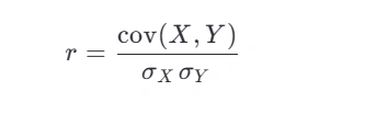
The Pearson Correlation Coefficient (PCC) measures the linear relationship between two datasets X and Y :
Where
cov(X,Y) is the covariance,
σX and σY are standard deviations.
Traditionally, you’d need all data points upfront. But in real-time systems—like live sports dashboards—you can’t wait.
Why Real-Time Correlation Matters: A Live Sports Analytics Example
Imagine you’re a data engineer for an NBA analytics team. During a live game, your system tracks:
Player A’s shot attempts per minute
Team B’s defensive pressure index (a real-time metric based on opponent positioning)
Coaches want to know instantly: “Does increased defensive pressure reduce this player’s shooting frequency?”
Waiting until halftime isn’t an option. You need live correlation updates after every new data point—within milliseconds.
This is where online (streaming) correlation shines.
Challenges of Real-Time Calculation
Naively recalculating PCC from scratch after each new observation leads to:
O(n) time per update → too slow for high-frequency data
Redundant recomputation of means and sums
Memory bloat if storing all historical points
The solution? An incremental algorithm that updates sufficient statistics on the fly.
Efficient Online Algorithm for Pearson Correlation
We maintain five running values:
n : count of observations
sumx,sumy : running sums
sumx2,sumy2 : sums of squares
sumxy : sum of products
Using these, we compute:
Means: xˉ=sumx/n
Variances and covariance
This gives O(1) per update and O(1) memory.
Complete Implementation with Live Simulation
import math
import random
import time
from typing import Optional

class OnlinePearsonCorrelation:
    """
    Computes Pearson correlation coefficient in real time using a
    numerically stable, one-pass method (Welford-style for covariance).
    O(1) per update.
    """

    def __init__(self):
        self.n = 0
        self.mean_x = 0.0
        self.mean_y = 0.0
        # M2X: Sum of squared differences from the current mean for x (proportional to variance)
        self.M2X = 0.0
        # M2Y: Sum of squared differences from the current mean for y (proportional to variance)
        self.M2Y = 0.0
        # CXY: Sum of products of differences from the current means (proportional to covariance)
        self.CXY = 0.0

    def update(self, x: float, y: float) -> None:
        """Add a new (x, y) observation and update statistics using the stable method."""
        self.n += 1

        # New delta for x and y
        delta_x = x - self.mean_x
        delta_y = y - self.mean_y

        # Update means
        self.mean_x += delta_x / self.n
        self.mean_y += delta_y / self.n

        # New delta after mean update (for stable variance calculation)
        delta_x2 = x - self.mean_x
        delta_y2 = y - self.mean_y

        # Update M2X, M2Y, and CXY
        self.M2X += delta_x * delta_x2
        self.M2Y += delta_y * delta_y2
        self.CXY += delta_x * delta_y2 # Stable cross-product

    def correlation(self) -> float:
        """Return current Pearson correlation coefficient."""
        if self.n < 2:
            return 0.0  # Not enough data

        # Numerator is the current Sum of Products (proportional to covariance)
        numerator = self.CXY

        # Denominators are the current Sum of Squares (proportional to variance)
        denom_x = self.M2X
        denom_y = self.M2Y

        # Check for zero variance
        if denom_x <= 1e-9 or denom_y <= 1e-9: # Use a small epsilon for float comparison
            return 0.0

        # Correlation r = Covariance / (StdDev_x * StdDev_y)
        # r = CXY / sqrt(M2X * M2Y)
        return numerator / (denom_x * denom_y) ** 0.5

    def reset(self) -> None:
        """Clear all stored statistics."""
        self.__init__()


# --- Live Simulation: NBA Game Analytics (Modified to use the fixed class) ---

def simulate_basketball_stream():
    """Simulate real-time player shot attempts vs defensive pressure."""
    correlator = OnlinePearsonCorrelation()

    print(" Live Correlation: Shot Attempts vs Defensive Pressure (Numerically Stable)")
    print("-" * 68)

    for minute in range(1, 13):  # Simulate 12-minute quarter
        # Simulate data: higher pressure slightly reduces shots
        pressure = random.uniform(0.3, 0.9)
        base_shots = 2.5
        # Introduce a negative relationship: higher pressure -> fewer shots
        shots = max(0, base_shots - 1.8 * pressure + random.gauss(0, 0.3))

        correlator.update(shots, pressure)
        corr = correlator.correlation()

        print(f"Minute {minute:2d} | N: {correlator.n:2d} | Shots(X): {shots:4.1f} | Pressure(Y): {pressure:.2f} | "
              f"Correlation(r): {corr:6.3f}")
        time.sleep(0.1) # Faster simulation for demonstration

    print("\n Insight: The negative correlation (r < 0) suggests pressure reduces shooting efficiency.")


if __name__ == "__main__":
    simulate_basketball_stream()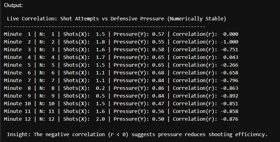
Key Features
Handles edge cases (insufficient data, zero variance)
Numerically stable for streaming data
Resettable for new game segments (e.g., quarters)
Best Practices and Performance Tips
Avoid division by zero: Always check variance denominators.
Use double precision: Prevents floating-point drift in long streams.
Reset per context: In sports, reset correlation each quarter or player substitution.
Combine with smoothing: For noisy data, apply exponential moving averages before correlation.
Validate with batch: Periodically cross-check against full recomputation for debugging.
Conclusion
Real-time Pearson correlation isn’t just theoretical—it’s a game-changer in live domains like sports, finance, and industrial monitoring. By maintaining running sums instead of raw data, you achieve constant-time updates and minimal memory usage. The next time a coach asks, “Is this defensive strategy working right now?”—you’ll have the answer before the next timeout. Master streaming statistics. Ship insights at the speed of reality.
Join the conversation! Your thoughts help the community grow.